Depth image coding using piecewise-linear functions

[chapter:depth_compression] This chapter proposes a novel depth image coding algorithm which concentrates on the special characteristics of depth images: smooth regions delineated by sharp edges. The algorithm models these smooth regions using piecewise-linear functions and sharp edges by a straight line. To define the area of support for each modeling function, we employ a quadtree decomposition that divides the image into blocks of variable size, each block being approximated by one modeling function containing one or two surfaces. The subdivision of the quadtree and the selection of the type of modeling function are optimized, such that a global rate-distortion trade-off is realized. Experimental results show that the described techniques improve the resulting quality of compressed depth images by up to 3 dB, when compared to a JPEG-2000 encoder.

Introduction

Previous work on depth image coding has used a transform-based algorithm derived from JPEG-2000 [92], [93] and MPEG encoders [94]. The key advantage of using a standardized video coding algorithm to compress depth images is the backward compatibility with already existing technology. However, transform coders have shown a significant shortcoming for representing edges without deterioration at low bit rates. Perceptually, such a coder generates ringing artifacts along edges that lead to errors in pixel positions, which appear as blurring within the depth signal-definition along the object borders. An alternative approach is to use triangular meshes [95], [96] to code depth maps. This alternative technique divides the image into triangular patches and approximates each patch by a linear function. If the data cannot be represented with a single linear function, smaller patches are used for that area. However, the placement of the patches is usually based on a regular grid, such that a large number of small patches are generated along edges.

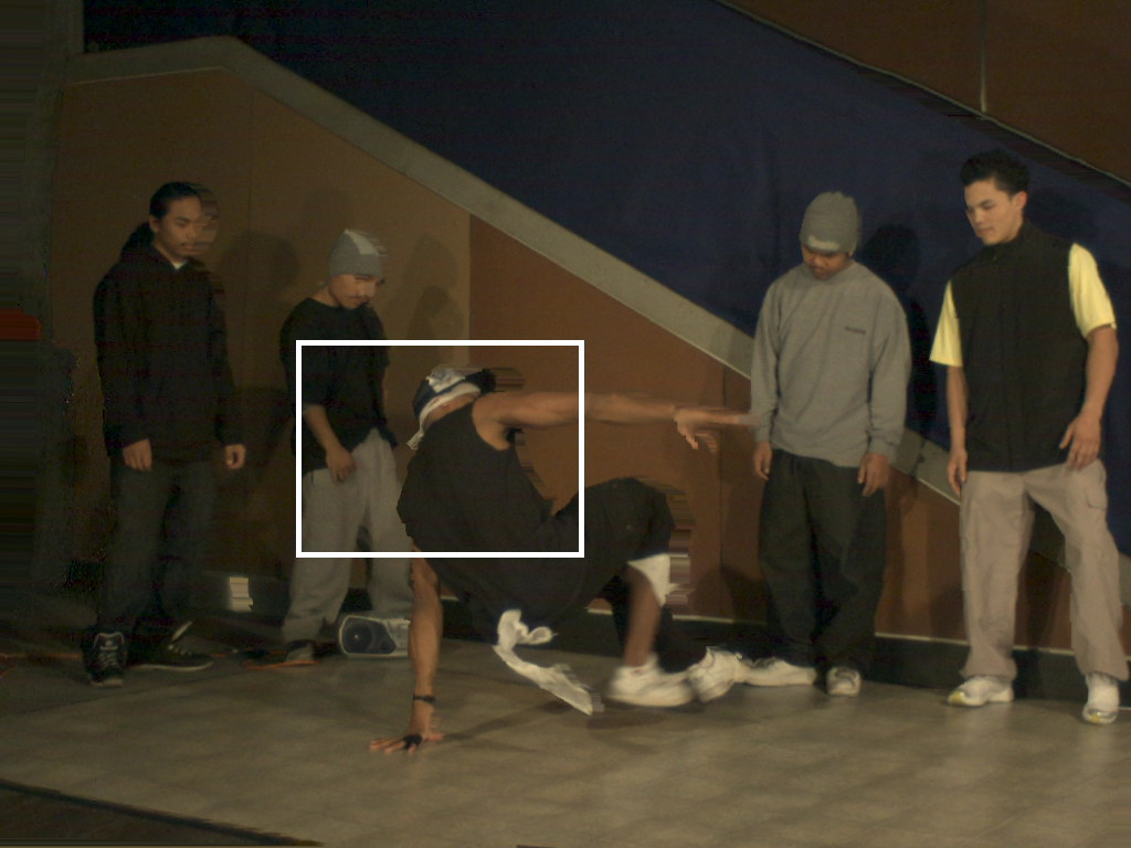
The characteristics of depth maps significantly differ from normal textured images (see Figure 6.1). For example, since a depth map explicitly captures the 3-D structure of a scene, large parts of typical depth images represent object surfaces. As a result, the input depth image contains various areas of smoothly changing grey levels. Furthermore, at the object boundaries, the depth map incorporates step functions, i.e., sharp edges.

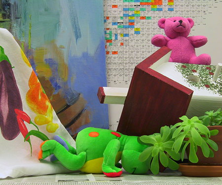
Figure 6.1 Example texture image (left) and the corresponding depth map (right). A typical depth image contains regions of linear depth changes bounded by sharp discontinuities.

Following these observations, we propose to model depth images by piecewise-linear functions which are separated by straight lines. For this reason, we are interested in an algorithm that efficiently extracts the sparse elements of the geometrical structures within the depth signal, yielding a compact representation and thus a low bit rate without significant distortion. Several contributions have considered the use of geometrical models to approximate images. Such a modeling function, the “Wedgelet” function [97], is defined as two piecewise-constant functions separated by a straight line. This concept was originally introduced as a means for detecting and recovering edges from noisy images, and was later extended to piecewise-linear functions, called “Platelet” [98] functions. To define the area of support of each modeling function, a quadtree segmentation of the image is used. The concept is to recursively subdivide the image into variable-size blocks and approximate each block with an appropriate model.

The framework used within this chapter for compression of 3D video signals is that we discuss depth-signal coding here independently from the textured video. Hence, we make an attempt to find an algorithm that well fits to the characteristics of the depth signal and we assume that the texture video is coded with any suitable video coder, such as H.264/MPEG-4 AVC. Considering this compression framework, we have adopted the “Wedgelet” and “Platelet” image-modeling method. In this way, we follow the idea developed to code images using piecewise polynomials [99] as modeling functions. More particularly, we consider four different piecewise-linear functions for modeling. The first and second modeling functions, which are a constant and linear function, respectively, have been found suitable to approximate smooth regions. The third and fourth modeling functions attempt to capture depth discontinuities, using two constant functions or two linear functions separated by a straight line. The proposed four modeling functions are used to approximate the entire image. To this end, the depth image is subdivided into variable-size blocks, using a quadtree decomposition. An independent modeling function is subsequently selected for each node. The selection of the most appropriate function is performed using a cost function that balances both rate and distortion. In a similar way, we employ an equivalent cost function that determines the optimal block sizes employed within the quadtree. Our results show that the proposal yields up to 1-3 dB PSNR improvement over a JPEG-2000 encoder.

This chapter is organized as follows. In the next section of this chapter, we define the previously introduced piecewise-linear modeling functions. Afterwards, Section 6.3 describes the bit-allocation strategy for mapping the model function outputs to code words, using rate-distortion principles. Experimental results are provided in Section 6.4 and the chapter concludes with Section 6.5.

Geometric modeling of depth images

Overview of the depth image coding algorithm

In this section, we present a novel approach for depth image coding using the piecewise-linear functions mentioned in Section 6.1. The concept followed is to approximate the image content with modeling functions. In our framework, we use two classes of modeling functions: a class of piecewise-constant functions and a class of piecewise-linear functions. For example, flat surfaces that show smooth regions in the depth image can be approximated by a piecewise-constant function. Similarly, planar surfaces of the scene like the ground plane and walls, appear as regions of gradually changing grey levels in the depth image. Hence, such a planar region can be approximated by a single linear function. To identify the location of these surfaces in the image, we employ a quadtree decomposition (see Figure 6.2), which recursively divides the image into variable-size blocks, i.e., nodes of different size, according to the degree of decomposition.

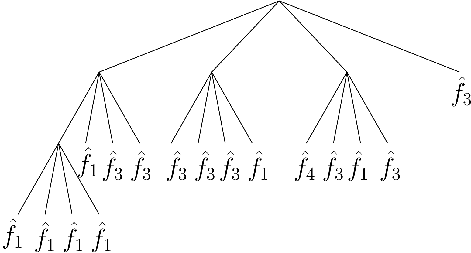
Figure 6.2 Example of quadtree decomposition. Each block, i.e., nodes, of the quadtree is approximated by one modeling function.

In some cases, the depth image within one block can be approximated with one modeling function. If no suitable approximation can be determined for the block, it is subdivided into four smaller blocks. To prevent that too many small blocks are required along a discontinuity, we divide the block into two regions separated by a straight line. Each of these two regions is coded with an independent function. Consequently, the algorithm chooses between four modeling functions for each leaf as follows.

• Modeling function \(\hat{f}_1\): This function approximates the block content with a constant function.

• Modeling function \(\hat{f}_2\): This function approximates the block content with a linear function.

• Modeling function \(\hat{f}_3\): This function subdivides the block into two regions separated by a straight line and approximates each region with a constant function (a wedgelet function);

• Modeling function \(\hat{f}_4\): This function subdivides the block into two regions separated by a straight line and approximates each region with a linear function (a platelet function);

The selection of a particular modeling function is based on a rate-distortion criterion that is described in Section 6.3.1. This criterion trades-off the distortion and rate of the individual functions.

Modeling-function definitions

In this section, we define the four different modeling functions \(\hat{f}_j\), for \(j\in\{1,2,3,4\}\), used to approximate each quadtree block. To model the depth signal within each block, we focus on finding a compression scheme that can compactly represent smooth blocks as well as boundaries (contours) of objects. First, to approximate smooth blocks, we employ a simple constant function \(\hat{f}_1(x,y)=\alpha_0\). Second, to approximate gradually changing object surfaces, we use a piecewise-linear function \(\hat{f}_2\), which defined by \[\begin{array}{ll} \hat{f}_2(x,y)= (\beta_0+\beta_1 x+\beta_2 y), & \textrm{for }(x,y) \in S. (1) \end{array}\] Third, to properly approximate blocks containing sharp edges, we segment those blocks into two regions \(A\) and \(B\) divided by a straight line of arbitrary direction. Each region is subsequently approximated by one modeling function. To define the position and direction of the subdivision-line, we connect two pixels, \(P_1\) and \(P_2\), located at two different sides of the block. For coding the key parameters of this line, instead of saving the coordinates of both marker points, we use two indexes \(i_1\) and \(i_2\) addressing the location of \(P_1\) and \(P_2\). The index is defined such that all pixels directly surrounding the block are scanned in a clockwise fashion (see Figure 6.3).

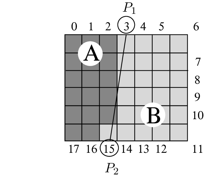
Figure 6.3 An example edge line that divides a quadtree block into two regions \(A\) and \(B\), using pixels \(P1\) (index 3) and \(P2\) (index 15) as marker points.

To determine if a pixel belongs to region \(A\) or \(B\), we use a numerical test known as the orientation test in computational geometry applications.

The two resulting regions \(A\) and \(B\) can be approximated by either a wedgelet function, or a platelet function. A wedgelet function is composed of two piecewise-constant functions over two regions \(A\) and \(B\), separated by a straight line, and can be defined as \[\hat{f}_{3}(x,y)=\left\{ \begin{array}{ll} \hat{f}_{3A} (x,y) = \gamma_{0A}, & \textrm{for } (x,y) \in A, \\ \hat{f}_{3B} (x,y) = \gamma_{0B}, & \textrm{for } (x,y) \in B. \end{array} \right. (6.2)\] Similarly, a platelet function is composed of two planar surfaces covering two different regions and separated by a straight edge (waterfall), and is defined by \[\hat{f}_4(x,y)=\left\{ \begin{array}{ll} \hat{f}_{4A} (x,y) = \theta_{0A} + \theta_{1A}x+\theta_{2A}y, & \textrm{for } (x,y) \in A, \\ \hat{f}_{4B} (x,y) = \theta_{0B} + \theta_{1B}x+\theta_{2B}y, & \textrm{for } (x,y) \in B. \end{array} \right. (6.3)\] Figure [fig:modelexample] depicts example patterns for each modeling function \(\hat{f}_1\), \(\hat{f}_2\), \(\hat{f}_3\) and \(\hat{f}_4\).

(a) (b) (c) (d)

Figure 6.4 (a)-(d) Examples of functions \(\hat{f}_1\), \(\hat{f}_2\), \(\hat{f}_3\) and \(\hat{f}_4\), respectively.

Let us now specify the computation of the function coefficients.

Estimation of model coefficients

The objective of the estimation step is to calculate the coefficients of the modeling functions subject to a constraint. We employ a constraint that minimizes the approximation error between the original depth signal in a block and the corresponding approximation. Specifically, the approximation error is the Mean Squared Error (MSE) over the block where the model applies to. Let us divide the estimation of the modeling function into two sections: one for the constant functions, and one for the linear functions.

A. Coefficient estimation for modeling the constant functions \(\hat{f}_1\) and \(\hat{f}_2\).

For \(\hat{f}_1(x,y)=\alpha_0\), only one coefficient \(\alpha_0\) has to be computed. Practically, the coefficient \(\alpha_0\) that minimizes the MSE between \(f\) and \(\hat{f}_1\) simply corresponds to the mean value of the original data block, which leads to the computation of \(\alpha_0=\frac{1}{n\times n}\sum_{x,y\in S} f(x,y)\).

For \(\hat{f}_2\), the function should approximate blocks that contain a gradient. In order to determine the three coefficients \(\beta_0\), \(\beta_1\) and \(\beta_2\) of the linear function \(\hat{f}_2(x,y)=\beta_0+\beta_1 x+\beta_2 y\), a least-squares optimization is used. This optimization minimizes the sum of squared differences between the depth image \(f(x,y)\) and the proposed linear model. Accordingly, coefficients \(\beta_0\), \(\beta_1\) and \(\beta_2\) are determined such that the error \[\label{lms} e_2(\beta_0,\beta_1,\beta_2)= \sum _{x=1} ^{n} \sum _{y=1} ^{n} (\beta_0+\beta_1x+\beta_2 y-f(x,y) )^2 (6.4)\] is minimized, where \(n\) denotes the node size expressed in pixels. This error function \(e_2(\beta_0,\beta_1,\beta_2)\) is minimal when the gradient function crosses zero, hence \(||\nabla e_2 ||=0\). When taking the partial derivatives with respect to \(\beta_0,\beta_1\) and \(\beta_2\) of this equation, we find a set of linear equations ¹⁶ specified by \[\left( \begin{array}{ccc} t & u & v \\ u & t & v \\ v & v & n^2 \end{array} \right) \left( \begin{array}{c} \beta_1\\ \beta_2\\ \beta_0 \end{array} \right) = \left( \begin{array}{c} \sum_{x=1} ^{n} \sum_{y=1} ^{n} xf(x,y)\\ \sum_{x=1} ^{n} \sum_{y=1} ^{n} yf(x,y)\\ \sum_{x=1} ^{n} \sum_{y=1} ^{n} f(x,y) \end{array} \right), (6.5)\] with \[\textstyle t=\frac{n^2(n+1)(2n+1)}{6},\quad u=\frac{n^2 (n+1)^2}{4}, \textrm{ and } v=\frac{n^2(n+1)}{2}. (6.6)\] Since the matrix at the left side of the equation system is constant, it is possible to pre-compute and store the inverse for each size of the square (quadtree node). This enables to compute the coefficients \(\beta_0,\beta_1,\beta_2\) with a simple matrix multiplication.

B. Coefficient estimation for modeling the linear functions \(\hat{f}_3\) and \(\hat{f}_4\).

For the wedgelet \(\hat{f}_3\) and platelet \(\hat{f}_4\) functions, we have to determine not only the model coefficients, but also the separation line. For each model, we aim at approximating the depth value \(f(x,y)\) with two functions in the supporting areas \(A\) and \(B\). Each area is delineated by a subdividing line \(P_1P_2\), as defined by points \(P_1\) and \(P_2\) (see Figure 3.3). The best set of coefficients for the wedgelet \(\hat{f}_3\) and platelet \(\hat{f}_4\) functions are those coefficient values that minimize the approximation errors \[e_3 = ||f-\hat{f}_{3A} ||^2 + ||f-\hat{f}_{3B} ||^2 \quad \textrm { and } \quad e_4 =||f-\hat{f}_{4A} ||^2 + ||f-\hat{f}_{4B} ||^2, (6.7)\] respectively. These minimizations cannot be solved directly for the following reason. Without knowing the subdivision boundary between the two regions, it is not possible to determine the model coefficients. On the other hand, it is not possible to identify the subdivision line as long as the region coefficients are unknown. To overcome this mutual dependence, we first identify the separation line. For this reason, the coefficient estimation is initialized by testing every possible line that divides the block into two areas. This step provides a candidate subdivision line \(P_1^c P_2^c\) and two candidate regions \(A^c\) and \(B^c\). Subsequently, the wedgelet and platelet coefficients are computed over the candidate regions using the average pixel value and a least-squares minimization, respectively. At the end of the exhaustive search for each function \(\hat{f}_3\) and \(\hat{f}_4\), the best fitting model is selected. The major advantage of this technique is that it leads to the optimal set of coefficients that minimizes the least-squares error between the model and the image block. Table 6.1 shows a summary of possible modeling functions of the previous subsections to approximate each block of the quadtree and their corresponding coefficient-estimation techniques.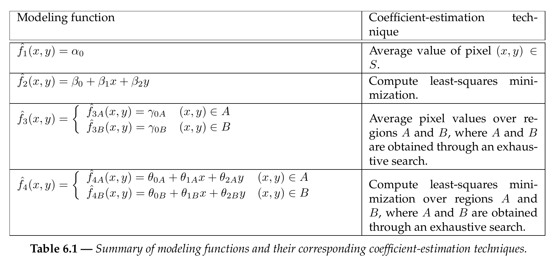

Bit-allocation strategy

This section provides details about the bit-allocation strategy that optimizes the coding in a rate-distortion sense. Lossy compression is a trade-off between rate and distortion. Considering our lossy encoder/decoder framework, our aim is to optimize the compression. This is realized by specifying an objective Rate-Distortion (R-D) constraint. There are three coding and modeling parameters that influence this trade-off.

• Quadtree decomposition. To accurately approximate a block that shows fine details, the quadtree decomposition recursively subdivides the block into smaller blocks. However, additional subdivisions lead to a higher bit rate. Therefore, an appropriate subdivision criterion is required, that prevents the creation of many small blocks.

• Selection of modeling functions. There are four different modeling functions \(\hat{f}_j,\ j\in\{1,2,3,4\}\), to approximate a depth pixel block. Each modeling function has a different approximation accuracy, but also different complexity (thus rate). Therefore, an appropriate model has to be selected that balances both rate and model distortion.

• Quantization step size. The quantization process in the encoder is covered by a variable quantization accuracy of the model coefficients. Thus, each function coefficient is quantized such that the model approximates the depth with a predetermined accuracy. In our case, the involved quantization step size is adapted to the required R-D constraint.

Concluding, the primary problem is to adjust each of the above parameters such that the objective R-D constraint is satisfied. To optimize these parameters in an R-D sense, a possible approach is to define a cost function that combines both rate \(R_i\) and distortion \(D_i\) of the image \(i\). Typically, for this problem, the Lagrangian cost function \(J(R_i)\) is used with \[J(R_i) = D_i(R_i)+ \lambda R_i, (6.8) \label{eq:lagrangian}\] where \(R_i\) and \(D_i\) represent the rate and distortion of the image, respectively, and \(\lambda\) is a weighting factor that controls the rate-distortion trade-off. For example, for \(\lambda=0\), we obtain a signal reconstructed at the lowest distortion and highest bit rate achievable. In the opposite case, for \(\lambda=\infty\), the signal is compressed at the lowest rate and highest distortion. To achieve an optimal encoding, the Lagrangian cost function \(J(R_i)\) should be minimized. This cost function is minimized when the derivative is set to \(0\), which yields \[\lambda= - \frac{ \partial{ D(R_i)} } {\partial{ R_i}}. (6.9)\] Thus, the optimal encoding is obtained when compressing the image at an operation point that has a constant slope \(-\lambda\) at the convex hull of the R-D points (see Figure 6.5).

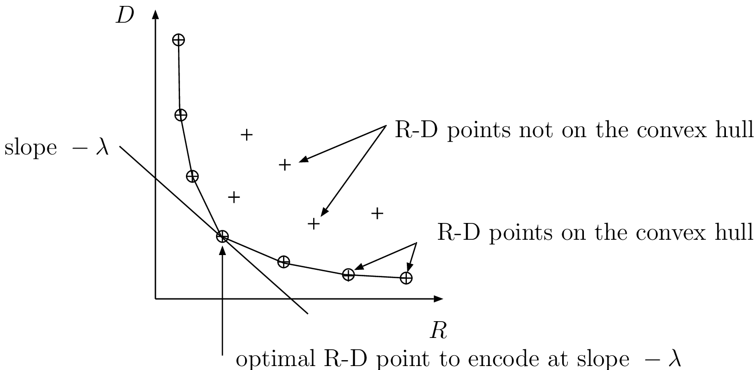Figure 6.5 Rate-distortion plane and convex hull of the R-D points.

Additionally, it can be shown that for an optimal encoding, not only the image must be encoded at constant R-D slope \(-\lambda\), but also for each independent sub-image [100]. As a consequence, the key principle followed in the discussed bit-allocation strategy is to adjust coding and modeling parameters (i.e., quadtree decomposition, model selection and quantizer step size), such that the image and also each quadtree block is encoded at a constant slope \(-\lambda\).

However, optimizing all parameters in a single iteration would be highly complicated. For example, without a given quadtree segmentation, it is not possible to select an appropriate modeling function for each quadtree block. To come to a feasible solution for this optimization problem, we divided the optimization procedure in three steps. We first assume that an optimal quadtree segmentation and coefficient quantizer setting is provided. Using this information, the selection of modeling functions for each quadtree block can be performed. Then, we describe a method to optimize the quadtree decomposition and finally, we optimize the quantizer setting. The complete solution will be developed later.

Modeling function selection

In Section 6.2.2, it was explained that a quadtree block can be approximated by four different modeling functions \(\hat{f}_1\), \(\hat{f}_2\), \(\hat{f}_3\) and \(\hat{f}_4\). The objective is not only to select the most appropriate modeling function, but also to incorporate this choice in the overall R-D constraint. The function mentioned in Equation (6.8) represents the global cost function for the image \(i\). However, the objective is now to select for each block the modeling function \(\hat{f}_j\), \(j\in\{1,2,3,4\}\), that minimizes the global coding cost \(D_i(R_i)+ \lambda R_i\).

Since the rate and distortion are additive functions over all blocks, an independent optimization can be performed for each block. This statement is valid because the modeling is performed for each block individually without a relationship to neighboring blocks. Therefore, for each block, the algorithm selects the modeling function that minimizes the Lagrangian R-D cost function according to \[\tilde{f} = {\mathop{\textrm arg\, min}}_{\hat{f}_j\in\{\hat{f}_1,\hat{f}_2,\hat{f}_3,\hat{f}_4 \} } ( D_m(\hat{f}_j) + \lambda R_m(\hat{f}_j) ) , (6.10) \label{eq:model_select}\] where \(R_m(\hat{f}_j)\) and \(D_m(\hat{f}_j)\) represent the rate and distortion resulting from using one modeling function \(\hat{f}_j\). In the implementation, the applied distortion measure is the squared error and the rate for each modeling function is derived from the predetermined quantizer setting.

Quadtree decomposition

Let us now provide more details about optimizing the quadtree decomposition. The objective is to obtain an optimal quadtree decomposition of an image in the R-D sense. Because the quadtree segmentation is not known in advance, the algorithm first segments the image into a full quadtree decomposition up to the pixel level. From this full tree, the algorithm aims at deriving a sub-tree that optimally segments and approximates the image in the R-D sense. To obtain an optimal tree decomposition of the image, a well-known approach is to perform a so-called bottom-up tree-pruning technique [101]. The concept is based on parsing the initial full tree from bottom to top and recursively prune nodes (i.e., merge blocks) of the tree according to a decision criterion. From earlier work, we have decided to adopt the already specified Lagrangian cost function for this purpose.

The tree-pruning algorithm is illustrated by Figure 6.6 and can be described as follows.

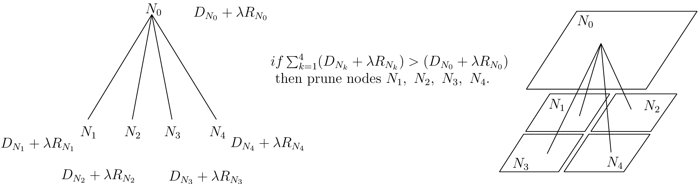
Figure 6.6 Illustration of a bottom-up tree-pruning procedure.

Consider four children nodes denoted by \(N_1\), \(N_2\), \(N_3\) and \(N_4\), that have a common parent node which is represented by \(N_0\). For each node \(k\), a Lagrangian coding cost \((D_{N_{k}} + \lambda R_{N_{k}}),\ k\in\{0,1,2,3,4\}\), can be calculated. Using the Lagrangian cost function, the four children nodes should be pruned whenever the sum of the four coding cost functions is higher than the cost function of the parent node. More formally written, the children nodes are pruned whenever the following condition holds \[\sum_{k=1}^4 (D_{N_{k}} + \lambda R_{N_{k}}) > (D_{N_{0}} + \lambda R_{N_{0}}). (6.11)\] When the children nodes are not pruned, the algorithm assigns the sum of the coding costs of the children nodes to the parent node. Subsequently, this tree-pruning technique is recursively performed in a bottom-up fashion. It has been proven [101] that such a bottom-up tree pruning leads to an optimally pruned tree, thus in our case to an R-D optimal quadtree decomposition of the image.

To estimate the bit rate at block level, we also include the side information required to code the node of the quadtree, the modeling function index and the bit rate resulting from using the modeling function. We address all three elements briefly. For the side information, we assume that the quadtree structure can be coded using one bit per node (one bit set to “1” or “0” to indicate that the node is subdivided or not). For the index, two bits per leaf are necessary to indicate which modeling function is used. The previous two aspects contribute to the bit rate. Hence, the rate \(R_{N_{k}}\) that is required to code one given node \(N_k\) can be written as \[R_{N_{k}}= 1 + 2 + R_m(\tilde{f}), (6.12)\] where \(R_m(\tilde{f})\) is the bit rate needed to code the best modeling function \(\tilde{f}\) (see Equation (6.10). The distortion \(D_{N_{k}}\) for one node \(N_k\) corresponds to the distortion introduced by the selected modeling function \(\tilde{f}\).

Quantizer selection

A criterion that selects the optimal quantizer is now described.

Up till now, we have discussed a scheme that subdivides the image into a full quadtree, optimizes the decomposition of the quadtree and optimally selects the modeling function for each node of tree. These optimizations were carried out under a predetermined quantizer setting. Now, the problem is to select the optimal quantizer, denoted \(\tilde{q}\), that yields the desired R-D trade-off. We propose to select the quantizer \(\tilde{q}\) out of a given set of possible scalar quantizers \(\{q_2,q_3,q_4,q_5,q_6,q_7,q_8\}\), operating at 2, 3, 4, 5, 6, 7 and 8 bits per level, respectively. To optimally select the quantizer, we re-use the application of the Lagrangian cost function and select the quantizer \(\tilde{q}\) that minimizes the Lagrangian coding cost of the image \(i\) according to \[\tilde{q} ={\mathop{\textrm arg\, min}}_{q_l\in\{q_2,q_3,q_4,q_5,q_6,q_7,q_8\} } D_i(R_i,q_l) + \lambda R_i(q_l). (6.13) \label{eq:quant_selection}\] Here, \(R_i(q_l)\) and \(D_i(R_i,q_l)\) correspond to the global rate \(R_i\) and distortion \(D_i(R_i)\), in which the parameter \(q_l\) is added to indicate the influence of the quantizer selection. To solve the optimization problem of Equation (6.13), the image is encoded using all possible quantizers \(\{q_2,q_3,q_4,q_5,q_6,q_7,q_8\}\) and the quantizer \(\tilde{q}\) is selected that yields the lowest coding cost for \(J_i(R_i,\tilde{q})=D_i(R_i,\tilde{q})+ \lambda R_i(\tilde{q})\).

Summary of the complete algorithm

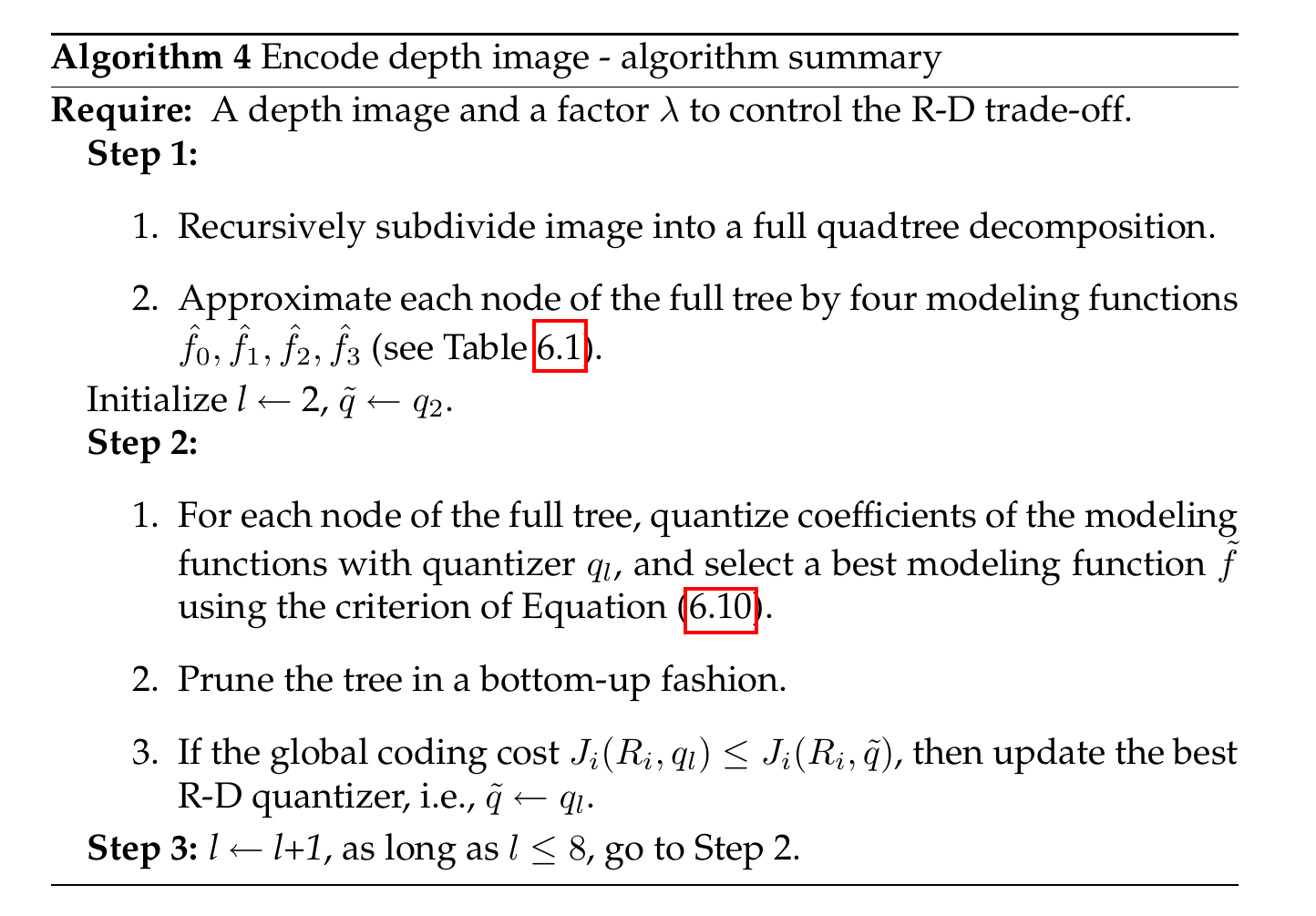
Since we have now defined how to select the modeling function, perform quadtree decomposition and know how to choose the quantizer setting, a complete algorithm for the joint optimization can be described. The algorithm requires as an input the depth image and a weighting factor \(\lambda\) that controls the R-D trade-off. The selection of the weighting factor \(\lambda\) that yields the desired bit rate can be calculated using a simple bisection search [102]. The image is first recursively subdivided into a full quadtree decomposition. All nodes of the tree are then approximated by four modeling functions \(\hat{f}_0\), \(\hat{f}_1\), \(\hat{f}_2\), \(\hat{f}_3\). In a second step, the coefficients of the modeling functions are quantized using one scalar quantizer \(q_l\). For each node of the full tree, an optimal modeling function \(\tilde{f}\) can now be selected using Equation (6.10). Employing the tree-pruning technique described in Section 6.3.2, the full tree is then pruned in a bottom-up fashion. Then, the previous step of the algorithm is repeated for all quantizers \(q_l\in\{q_2,q_3,q_4,q_5,q_6,q_7,q_8\}\) and the quantizer that leads to the lowest global coding cost is selected (see Equation (6.13)). Subsequently, for each leaf of the tree, the quantized zero-order coefficients \((\alpha_0,\beta_0,\gamma_{0A}, \gamma_{0B}, \theta_{0A}, \theta_{0B})\) are saved and because they are uniformly distributed, they are fixed-length coded. However, the first-order coefficients (\(\beta_1\), \(\beta_2\), \(\theta_{1A}\), \(\theta_{2A}\), \(\theta_{1B}\), \(\theta_{2B}\)) satisfy a Laplacian distribution. For this reason, we encode these coefficients using an adaptive arithmetic encoder. The pseudo-code of the complete algorithm is summarized in Algorithm 4.

Experimental results

In this section, we first present rate-distortion curves of the proposed depth image encoder. Second, the quality of rendered views synthesized using coded depth images is evaluated.

Coding experiments

Since this depth coding algorithm is completely new at the design time and there is no alternative, the performance was compared a number may be compared to a number of alternative image encoders, e.g., the Bandelet encoder [103], [104], the Contourlet encoder [105] or the Ridgelet encoder [106]. However, each of these alternatives employs a wavelet-based encoder as a reference. Because of the high coding performance of standard encoders such as the H.264/MPEG-4 AVC and JPEG-2000, these coders will be used for comparison.

A. Comparison with JPEG-2000

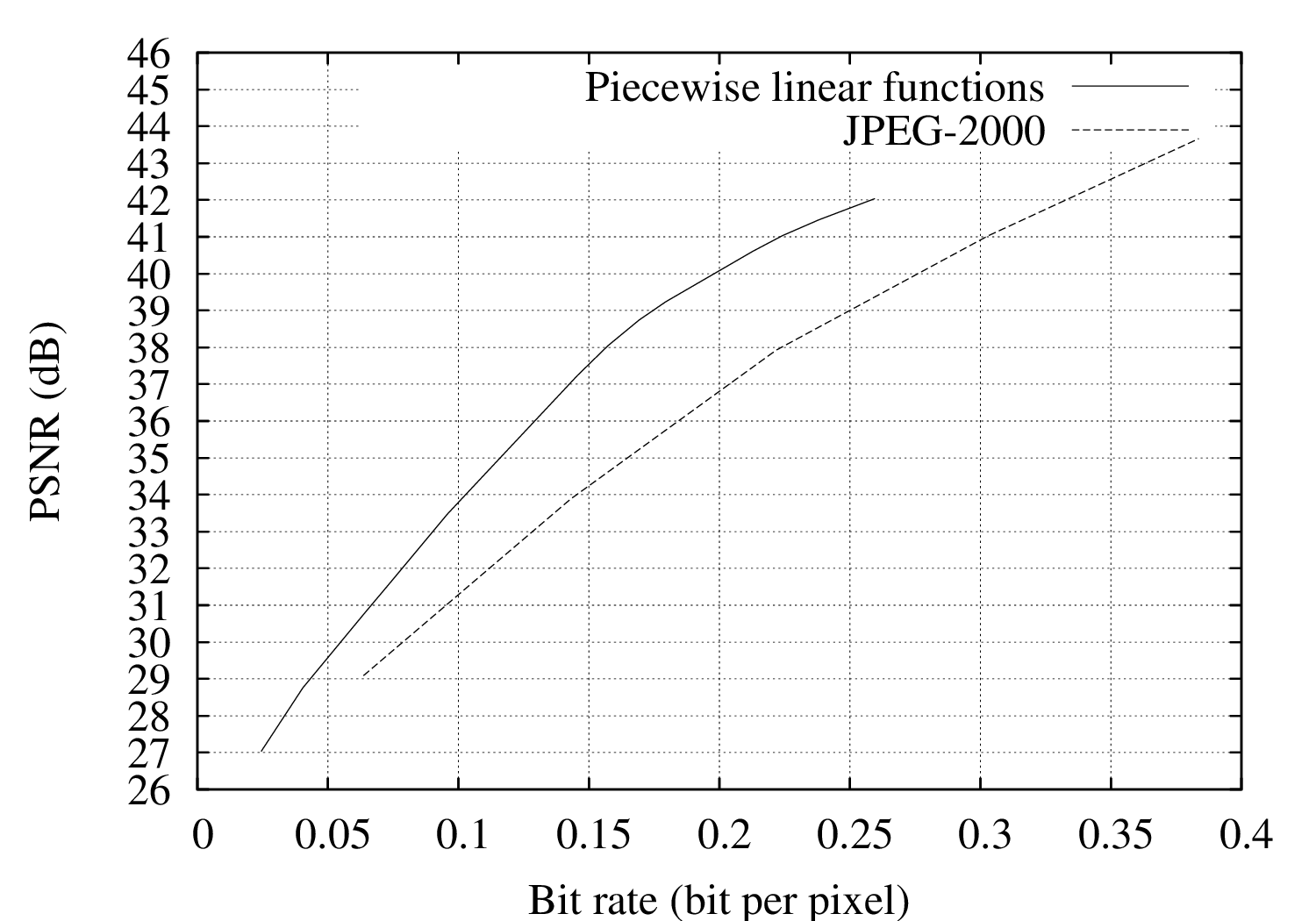
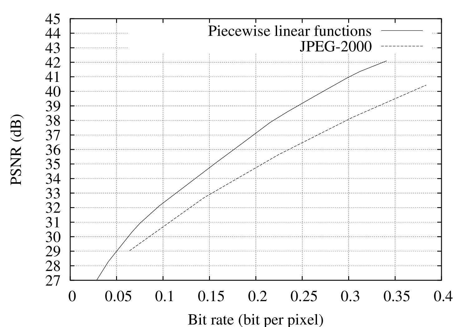
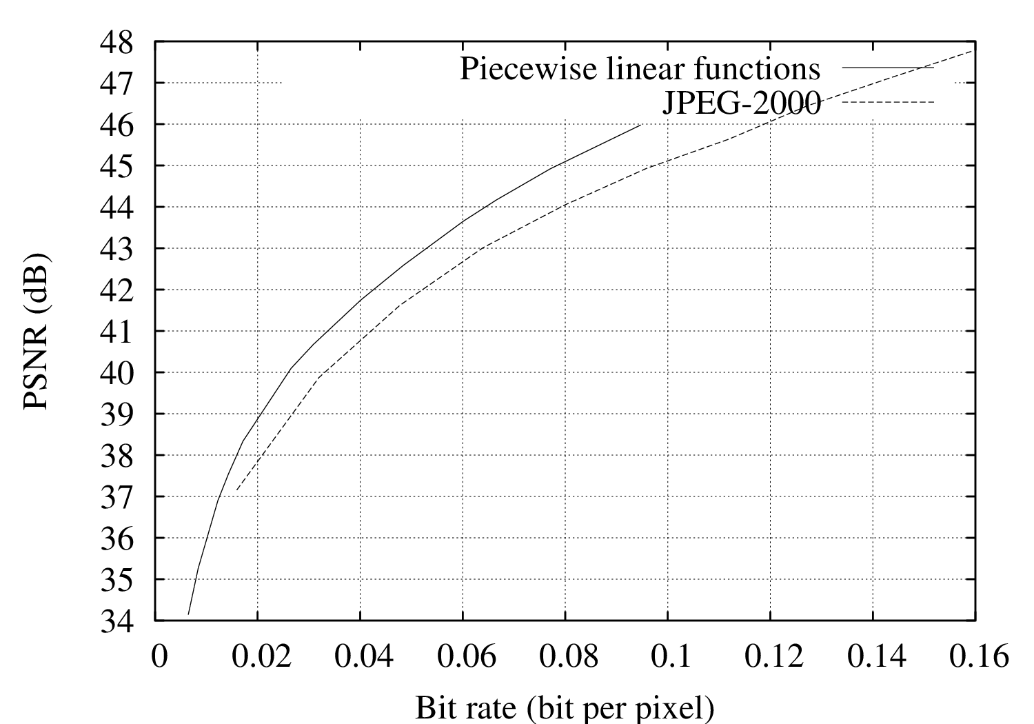
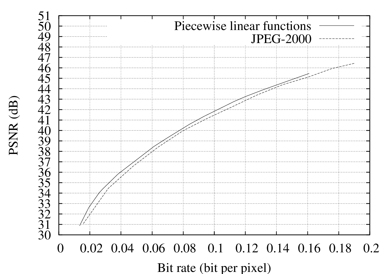
For evaluating the performance of the coding algorithm, experiments were carried out using the “Teddy”, “Cones”, “Breakdancers” and “Ballet” depth images.¹⁷ The R-D performance of the proposed encoder has been compared to a wavelet-based JPEG-2000 encoder [107]. Let us now examine the resulting rate-distortion curves of Figures 6.8(a), 6.8(b), 6.8(c) and 6.8(d). First, it can be observed that the proposed depth coder consistently outperforms the JPEG-2000 encoder. For example, considering the “Teddy” depth image, coding improvements over JPEG-2000 are as high as 2.5 dB and 3.3 dB at 0.1 and 0.2 bit per pixel, respectively. For the “Cones” depth image, an image-quality improvement of up to 2.8 dB at 0.3 bit per pixel can be observed. For the “Breakdancers” and “Ballet” images, a gain of 0.9 dB and 0.4 dB can be obtained at 0.04 bit per pixel, respectively.

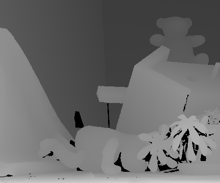
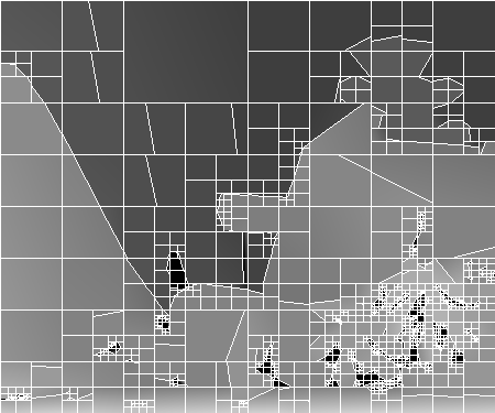
Let us now examine the subjective coding artifacts of the proposed depth coder. First, experiments have revealed that the proposed algorithm can approximate large smooth areas as well as sharp edges with a single node (see Figure 6.7). As a result, sharp edges are compactly encoded and accurately represented. An example is the left vertical edge in Figure 6.7(c).

(a) (b) (c)

Figure 6.7 (a) The original depth image “Teddy”. (b) The corresponding reconstructed depth image using the complete algorithm, (c) Superimposed nodes of the quadtree for the picture in (b). (Coding achieved with bit rate=0.12 bit/pixel and PSNR=36.1 dB).

Perceptually, our algorithm reconstructs edges of higher quality than the JPEG-2000 encoder. For example, the edge along the dancer in Figure 6.10(b) is accurately approximated when compared to the JPEG-2000 encoded signal (see Figure 6.10(c)), which is much more blurred.

(a)

(b)

Figure 6.8 Rate-distortion curves for the (a) “Teddy” and (b) “Cones” depth images, both for our algorithm and JPEG-2000.

(a)

(b)

Figure 6.9 Rate-distortion curves for the (a) “Breakdancers” and (b) “Ballet” depth images, both for our algorithm and JPEG-2000.

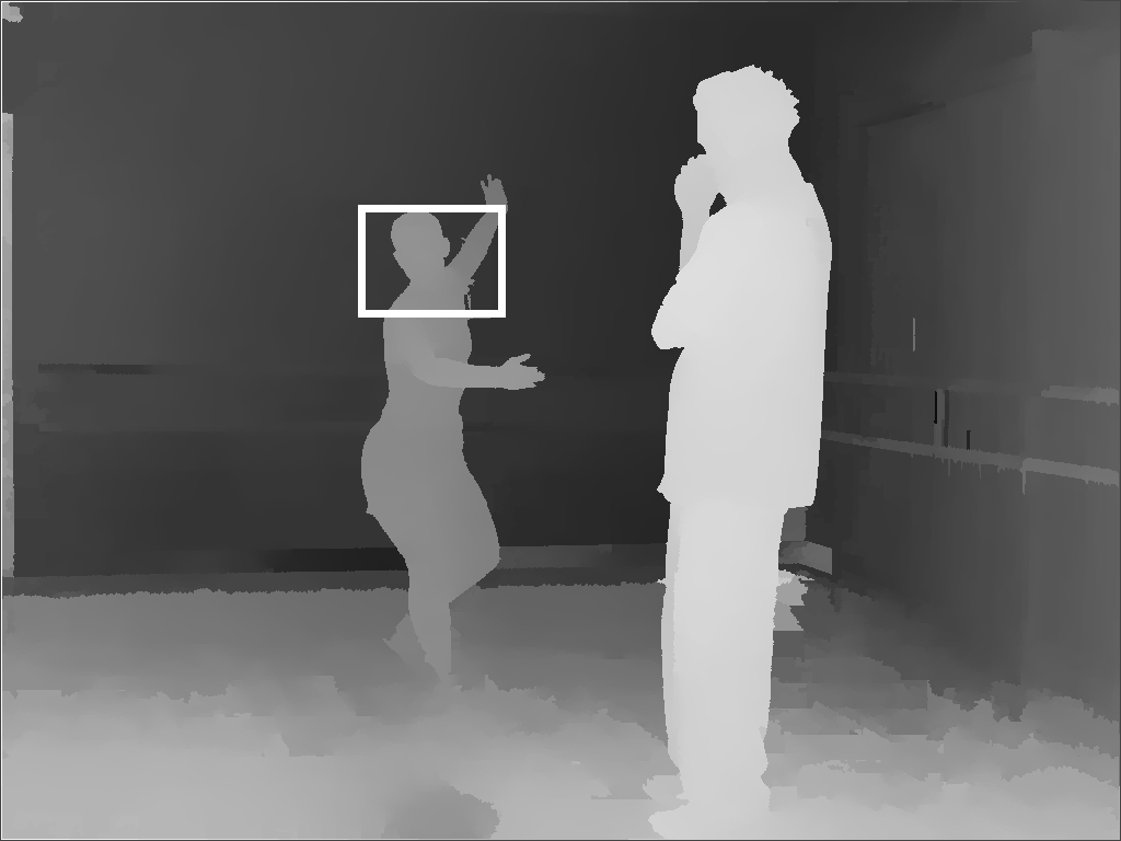
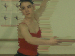
Figure 6.10 (a) “Ballet” depth image with a marked area. (b) The marked area coded with piecewise-linear functions at 35.8 dB PSNR. (c) Same area coded with JPEG-2000 at 35.5 dB PSNR. Both results are obtained at 0.038 bit/pixel.

Rendering experiments based on encoded depth

Let us now evaluate the quality of synthetic views rendered, using depth images encoded by the complete algorithm. The described experiment employs as input a depth image combined with the corresponding texture image and two neighboring texture views/images. To measure the rendering distortion, one approach consists of rendering a synthetic view at the position of a neighboring camera (same procedure as in Section 4.5). A rendering-distortion measure can be obtained by calculating the PSNR between the original and the rendered view. Practically, for this rendering PSNR evaluation, we have employed two neighboring texture views/images, from which the two resulting PSNR measures have been averaged. In Section 3.4.5, we have discussed the problem of selecting an appropriate objective rendering quality metric. Specifically, two rendered synthetic images with very different subjective qualities may show a similar objective PSNR quantity. This case will be illustrated by Figure 6.11. However, the PSNR was finally selected as a quality metric because it remains widely employed and the most broadly accepted metric by the research community. To evaluate the impact of depth compression on the rendering quality, the reference depth image is encoded at three different bit rates using two different depth-coders based on: (1) JPEG-2000 and (2) piecewise-linear functions. In this experiment, we investigate the impact of depth compression on the quality of the synthetic views. Therefore, the reference texture image is not encoded. The employed image rendering algorithm is the relief texture mapping algorithm which was presented in Section 4.2.3. Table 6.2 summarizes the rendering-quality measurements for the “Breakdancers” and “Ballet” sequences.

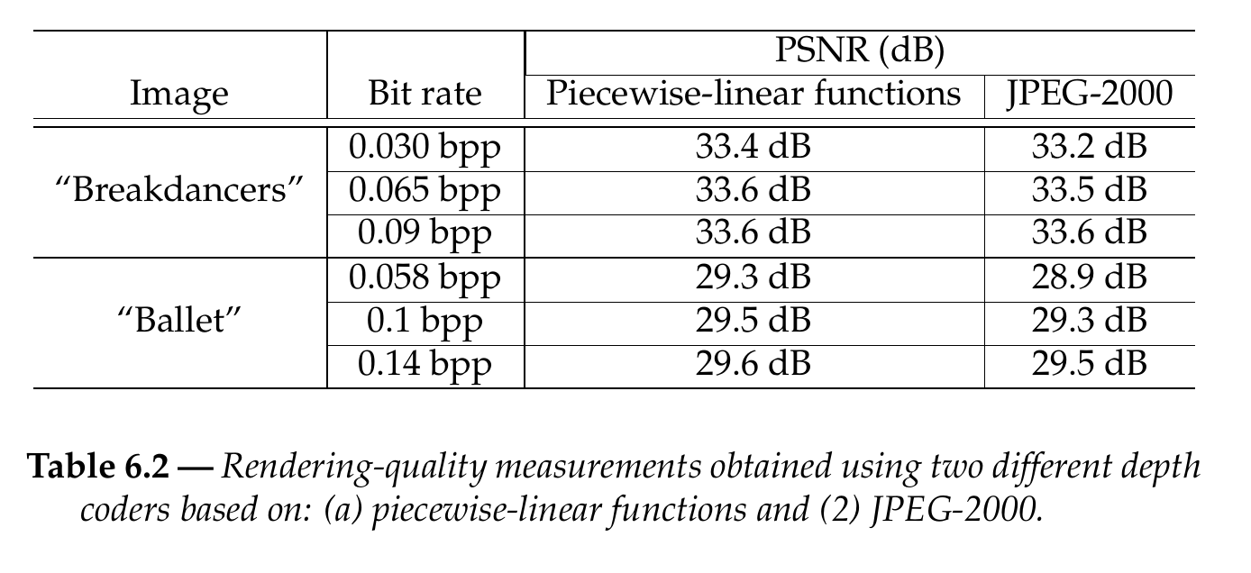
Let us now discuss the obtained rendering quality. First, it can be observed that the depth coder based on piecewise-linear functions consistently outperforms the JPEG-2000 coder in terms of rendering. For example, an image-quality improvement of up to 0.2 dB and 0.4 dB can be observed for the “Breakdancers” and “Ballet” sequences, respectively. As expected, the image-quality improvement is particularly significant at object borders. For example, the depth discontinuity along the edges of the lady dancer in the “Ballet” sequence is preserved (Figure 6.11(c)). At the opposite, a JPEG-2000 coder deteriorates depth discontinuities, resulting in rendering artifacts (Figure 6.11(a)). In this case, it should be noted that the rendering-distortion values of both images are comparable and equal to 29.5 dB and 29.3 dB. Hence, although both images show only a limited rendering-distortion difference of 0.2 dB, important visual differences can be observed. Similar conclusions can be drawn by observing synthetic images of the “Breakdancers” sequence (see Figure 6.12).

(a) (b)

(c) (d)

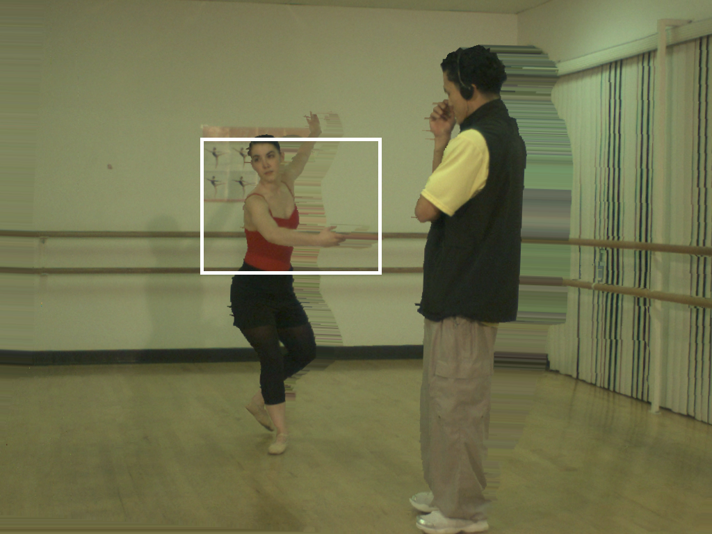
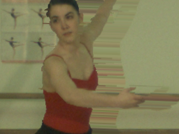
Figure 6.11(a) and (b) Synthetic image and corresponding magnified area rendered using a depth image encoded by a JPEG-2000 coder. (c) and (d) Synthetic image and corresponding magnified area rendered using a depth image encoded by a coder based on piecewise-linear functions. Both reference depth images are encoded at \(0.1\) bit per pixel.

(a) (b)

(c) (d)

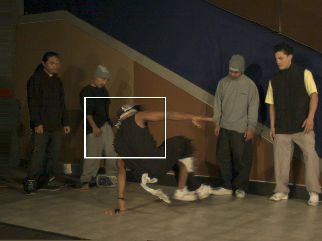
Figure 6.12 (a) and (b) Synthetic image and corresponding magnified area rendered using a depth image encoded by a JPEG-2000 coder. (c) and (d) Synthetic image and corresponding magnified area rendered using a depth image encoded by a coder based on piecewise-linear functions. Both reference depth images are encoded at \(0.03\) bit per pixel.

Comparisons with H.264/MPEG-4 AVC and MVC

Besides the coding performance comparisons with JPEG-2000, additional comparisons with two encoders based on H.264/MPEG-4 AVC were carried out in collaboration with P. Merkle from Fraunhofer HHI. In the discussed experiments, Merkle carried out the compression and the rendering of the multi-view sequences using the H.264/MPEG-4 AVC and MVC encoders, while the author performed the encoding of the depth image sequences using the proposed platelet-based encoder (also termed earlier as the coder based on piecewise-linear functions; in the remainder, we employ the platelet-based term to save text). To evaluate the compression efficiency of the platelet-based encoder, we have employed two different reference encoders. First, an H.264/MPEG-4 AVC encoder has been employed to compress the multi-view depth sequences. Note that the proposed platelet-based encoder does not exploit the temporal and spatial inter-view correlations. Thus, to obtain similar compression settings, the GOP size of the H.264/MPEG-4 AVC was set to 1 (intra-coding only). Second, an MVC encoder has been used for compressing the multi-view depth sequences. The compression settings of the MVC encoder have been initialized such that the CABAC and the rate control are enabled and that the motion search range is \(\pm 96\) pixels.

The first coding comparison [28] shows that the platelet-based encoder is outperformed by an H.264/MPEG-4 AVC intra-coding. However, experiments have also revealed that a lower coding efficiency does not imply a lower rendering quality. Specifically, the rendering-quality evaluation shows that a platelet-based encoder achieves an equal or better rendering quality, although its coding efficiency is lower than the effiency of H.264/MPEG-4 AVC intra-coding.

The second comparison [29] has revealed that also the MVC encoder yields a higher coding efficiency than a platelet-based encoder. This higher coding efficiency is obtained because the MVC encoder exploits the temporal and inter-view correlations. However, considering the “Breakdancers” sequence, the proposed depth encoder renders synthetic images with higher quality (when compared to an MVC depth encoder). For the “Ballet” sequence, the platelet-based encoder yields similar or slightly lower rendering quality. However, subjective evaluations of the rendered pictures show that the depth images encoded with a platelet-based encoder yield synthetic images with less rendering artifacts. For more details about the experimental settings and the experimental results, the reader is referred to the corresponding joint publications [28], [29].

Conclusions and perspectives

This chapter has resulted in a new coding algorithm for depth images that explicitly exploits the smooth properties of depth signals. Regions are modeled by piecewise-linear functions and they are separated by straight lines along their boundaries. The algorithm employs a quadtree decomposition to enable the coding of small details as well as large regions with a single node. The performance of the full coding algorithm can be controlled by three different coding and modeling aspects: the level of the quadtree segmentation, the overall coefficient-quantization setting for the image and the choice of the modeling function. All three aspects are controlled by a Lagrangian cost function, in order to impose a global rate-distortion constraint for the coding of the complete image. For typical bit rates (i.e., between 0.01 bit/pixel and 0.25 bit/pixel), experiments have revealed that the coder outperforms a JPEG-2000 encoder by 0.6 to 3.0 dB. Finally, we have shown that the proposed depth coder yields a rendering quality improvement of up 0.4 dB, when compared to a JPEG-2000 encoder. It has been reported by Farin et al. [27] that the coding system discussed in this chapter can be further improved. This improved coding performance is obtained by exploiting the inter-block redundancy within the quadtree. By decorrelating the remaining dependencies between each block, extra improvements of 0.3 to 1.0 dB can be obtained. Also, Merkle et al. have compared the proposed depth coder with an H.264/MPEG-4 AVC encoder (intra-coding). Experimental results have shown that an H.264/MPEG-4 AVC based coder slightly outperforms the coding of the proposed coder in bit rate. However, the result of this evaluation shows that the proposed coding system, as it is specialized on the characteristics of depth images, outperforms H.264/MPEG-4 AVC (intra-coding) in rendering quality.

Whereas the presented coding scheme is still at its early stage of development, it has the potential of significantly improving not only the depth compression performance, but also the rendering quality of synthetic images in a multi-view system. Given the promising results, it is interesting to extend the encoder for exploiting the temporal and spatial inter-view redundancy.

Finally, we briefly comment on the complexity of the proposed coding framework. It should be noticed that the search for the best modeling function is computationally expensive, but only carried out at the encoder. The corresponding decoder is very simple and can be executed on a regular platform. The second important function is the rate-distortion optimization. Given the consistency of depth images over time, it would be easy to use R-D optimized settings of the previous frame and refine those settings for the current frame. This would reduce the amount of computation significantly without sacrificing much performance.

References

[27] Y. Morvan, D. Farin, and P. H. N. de With, “Depth-image compression based on an R-D optimized quadtree decomposition for the transmission of multiview images,” in IEEE international conference on image processing, 2007, vol. 5, pp. V–105–V–108.
[28] P. Merkle, Y. Morvan, A. Smolic, K. Mueller, P. H. de With, and T. Wiegand, “The effect of depth compression on multi-view rendering quality,” in IEEE 3DTV conference: The true vision - capture, transmission and display of 3D video, 2008, pp. 245–248.
[29] P. Merkle, Y. Morvan, A. Smolic, K. Mueller, P. H. de With, and T. Wiegand, “The effects of multiview depth video compression on multiview rendering,” Signal Processing: Image Communication, vol. 24, nos. 1-2, pp. 73–88, January 2009.
[92] R. Krishnamurthy, B.-B. Chai, H. Tao, and S. Sethuraman, “Compression and transmission of depth maps for image-based rendering,” in IEEE international conference on image processing, 2001, vol. 3, pp. 828–831.
[93] M. Maitre and M. N. Do, “Joint encoding of the depth image based representation using shape-adaptive wavelets,” in IEEE international conference on image processing, 2008, vol. 1, pp. 1768–1771.
[94] C. Fehn, K. Schuur, P. Kauff, and A. Smolic, “Coding results for EE4 in MPEG 3DAV.” ISO/IEC JTC 1/SC 29/WG 11, MPEG03/M9561, March-2003.
[95] D. Tzovaras, N. Grammalidis, and M. G. Strintzis, “Disparity field and depth map coding for multiview image sequence,” in IEEE international conference on image processing, 1996, vol. 2, pp. 887–890.
[96] B.-B. Chai, S. Sethuraman, and H. S. Sawhney, “A depth map representation for real-time transmission and view-based rendering of a dynamic 3D scene,” in First international symposium on 3D data processing visualization and transmission, 2002, pp. 107–114.
[97] D. Donoho, “Wedgelets: Nearly minimax estimation of edges,” Annals of Statistics, vol. 27, no. 3, pp. 859–897, March 1999.
[98] R. M. Willett and R. D. Nowak, “Platelets: A multiscale approach for recovering edges and surfaces in photon-limited medical imaging,” IEEE Transactions on Medical Imaging, vol. 22, no. 3, pp. 332–350, 2003.
[99] R. Shukla, P. L. Dragotti, M. N. Do, and M. Vetterli, “Rate-distortion optimized tree-structured compression algorithms for piecewise polynomial images,” IEEE Transactions on Image Processing, vol. 14, no. 3, pp. 343–359, 2005.
[100] P. Prandoni, “Optimal segmentation techniques for piecewise stationary signals,” PhD thesis, Ecole Polytechnique Fédérale de Lausanne, Lausanne, Switzerland, 1999.
[101] P. A. Chou, T. D. Lookabaugh, and R. M. Gray, “Optimal pruning with applications to tree-structured source coding and modeling,” IEEE Transactions on Information Theory, vol. 35, no. 2, pp. 299–315, March 1989.
[102] A. Ortega and K. Ramchandran, “Rate-distortion methods for image and video compression,” IEEE Signal Processing Magazine, vol. 15, no. 6, pp. 23–50, 1998.
[103] E. L. Pennec and S. Mallat, “Sparse geometric image representations with bandelets,” IEEE Transactions on Image Processing, vol. 14, no. 4, pp. 423–438, 2005.
[104] G. Peyré and S. Mallat, “Discrete bandelets with geometric orthogonal filters,” in IEEE international conference on image processing, 2005, vol. 1, pp. I–65–8.
[105] M. N. Do and M. Vetterli, “The contourlet transform: An efficient directional multiresolution image representation,” IEEE Transactions on Image Processing, vol. 14, no. 12, pp. 2091–2106, 2005.
[106] M. N. Do and M. Vetterli, “The finite ridgelet transform for image representation,” IEEE Transactions on Image Processing, vol. 12, no. 1, pp. 16–28, 2003.
[107] M. Adams and F. Kossentini, “JasPer: A software-based JPEG-2000 codec implementation,” in IEEE international conference on image processing, 2000, vol. 2, pp. 53–56.