Multi-View Depth Image Based Rendering

This chapter focuses on the rendering of synthetic images using multiple views. First, two different rendering techniques are investigated: a 3D image warping and a mesh-based rendering technique. Each of these methods has its limitations and suffers from either high computational complexity or low image rendering quality. Afterwards, we present two novel image-based rendering algorithms addressing the aforementioned limitations. The first of these two algorithms is an alternative formulation of the relief texture algorithm which was adapted to the geometry of multiple views. The proposed technique avoids holes in the synthetic image and is suitable for execution on a standard Graphics Processor Unit. The second proposed algorithm represents an inverse mapping rendering technique which allows a simple and accurate re-sampling of synthetic pixels. Moreover, multiple techniques for properly handling occlusions are introduced. The chapter concludes with a quality evaluation of the obtained synthetic images when using the proposed rendering techniques.

Introduction

This section starts with reviewing image rendering techniques and their advantages and disadvantages with respect to 3D-TV and free-viewpoint video applications. For each technique, we consider the constituting stages in the multi-view video processing chain: acquisition, transmission and rendering of multi-view video. Afterwards, we describe two multi-view video systems, relying either on a strong calibration (Section 2.3) or a weak calibration (Section 2.4) of the multi-view setup. It is shown that both forms of calibration enable an efficient acquisition and rendering. However, in the last part of the introduction, it will become clear that the compression of multi-view video can be performed more efficiently when employing a strongly calibrated system. In the previous chapter, calibrated depth images were estimated for each view. Hence, the depth images and the calibration parameters can be beneficially employed for rendering synthetic images. Later in this thesis, the same rendering techniques are integrated into the coding loop for exploiting inter-view redundancy.

Review of image rendering techniques

Synthetic images can be rendered using either texture-only images, or using a combination of a 3D geometric model and texture images. Rendering techniques can be therefore classified according to their level of detail of the geometric description of the scene [60].

Rendering without geometry.

A first class of techniques considers the use of multiple views (N-texture) of the scene but does not require any geometric description of the scene. For example, Light Field [59] and Lumigraph [61] record a 3D scene by capturing all rays traversing a 3D volume using a large array of cameras. Each pixel of the virtual view is then interpolated from the captured rays using the positions of the input and virtual cameras. However, such a rendering technique implies the capturing of the video scene using a large camera array, i.e., oversampling of the scene. Considering the 3D-TV and free-viewpoint video applications, such an oversampling is inefficient because a large number of video streams needs to be transmitted.

Rendering with geometry.

A second class of techniques involves the use of a geometric description of the scene for rendering. One approach applies polygons to represent the geometry of the scene, i.e., the surface of objects [62]. Virtual images are then synthesized using a planar-texture mapping algorithm (see Section 2.4.2). However, the acquisition of 3D polygons is a difficult task. An alternative method is to associate a depth image to the texture image. Using a depth image, new views can be subsequently rendered using a Depth Image Based Rendering (DIBR) algorithm. DIBR algorithms include, among others, Layered Depth Image [63], view morphing [64], point-clouds [65] and image warping [66]. We refer to the technique of associating one depth with one texture image [8], [67], [68] as the N-depth/N-texture representation format. The two advantages of the N-depth/N-texture approach are that (1) the data format features a compact representation, and (2) high-quality views can be rendered. For these reasons, this data format provides a suitable representation format for 3D-TV and free-viewpoint video applications. Consequently, the N-depth/N-texture representation format was adopted in this thesis.

Acquisition and rendering using N-depth/N-texture

Two possible approaches can be distinguished to render images, using an N-depth/N-texture representation format.

Weakly calibrated cameras.

A first approach [69] allows to synthesize intermediate views along a chain of cameras. The algorithm estimates the epipolar geometry between each pair of successive cameras and rectifies the images pairwise (see Figure 4.1(a)). Disparity images are estimated for each pair of cameras (see Section 3.2). Next, synthetic views are interpolated using an algorithm similar to View Morphing [64]. This approach of working along a chain of cameras has two advantages. First, the acquisition is flexible because the epipolar geometry can be estimated without any calibration device [35]. Second, a real-time rendering implementation [69] based on a standard Graphics Processor Unit (GPU) is feasible and was even demonstrated. However, this rendering technique does not enable the user to navigate within the 3D scene. Instead, the viewer can only select a viewpoint that is located on the poly-line connecting all camera centers along the chain of cameras.

Strongly calibrated cameras.

An alternative method [8] employs a similar video capturing system composed of a set of multiple cameras. As opposed to the above approach, the cameras are fully calibrated prior to the capture session (see Figure 4.1(b)). Therefore, the depth can be subsequently estimated for each view. To perform view synthesis, given the depth information, 3D image warping techniques can be employed. As opposed to a weakly calibrated multi-view setup, a first advantage of this approach is that it enables the user to freely navigate within the 3D scene. Additionally, a second advantage is that the compression of a multi-view video can be performed more efficiently by employing all camera parameters, an aspect that we discuss in the next section.

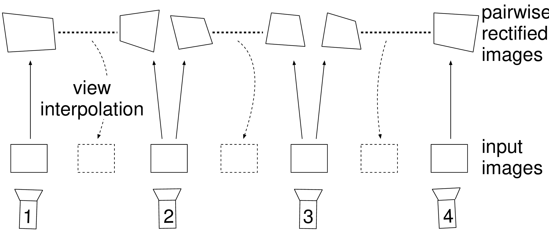
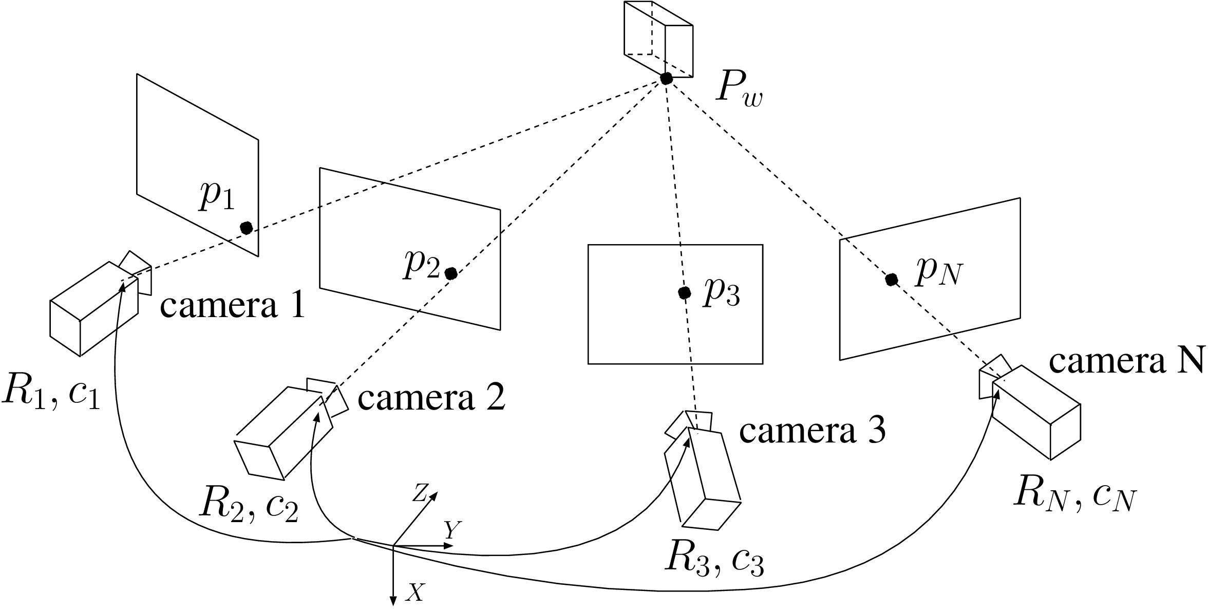
Figure 4.1 (a) For a weakly calibrated setup, the captured images are rectified pairwise. Disparity estimation and view interpolation between a pair of cameras is carried out on the rectified images. (b) For a strongly calibrated setup, the respective position and orientation of each camera is known. Depth images can therefore be estimated for each view and a 3D image warping algorithm can be used to synthesize virtual views.

Compression of N-depth/N-texture

To perform the compression of multi-view images, the redundancy between neighboring views should be exploited. To do so, one approach is to employ image rendering in a predictive fashion. More specifically, the rendering procedure can be employed to predict or approximate a view captured by a predicted camera. We describe in this section several rendering algorithms enabling the prediction of views. The integration of the rendering engine into the corresponding coding algorithm will be discussed in Chapter 5.

Weakly calibrated cameras.

To perform the prediction of an image using weakly calibrated cameras, the disparity image can be employed. However, we have shown in Section 3.2 that disparity images are estimated pairwise, i.e., between a left and right texture image. Consequently, the disparity image and the corresponding left texture image enable only the prediction of the right image. In other words, it is not possible to perform the prediction of other views than the right image.

Strongly calibrated cameras.

Alternatively, using a strongly calibrated camera setup, a depth image can be calculated for each view. As opposed to the disparity image that provides the pairwise disparity between a left and right image, a depth image indicates the 3D-world depth coordinates shared by all views. Therefore, it is possible to synthesize a virtual view at the position of any selected camera, thereby enabling the prediction of multiple views using one reference view only. Considering the problem of compression, a strongly calibrated multi-view acquisition system would be highly favorable.

Whereas image rendering has been an active field of research for multimedia applications [16], limited work has been focused on image rendering in a multi-view coding framework. Two recent approaches have employed either a direct projection of pixels onto the virtual image plane [8], or a method known as point-clouds rendering [70]. Both techniques are similar to the 3D image warping algorithm, so that they also suffer from known stair-case artifacts and holes (undefined pixels). An accurate prediction of views requires an accurate image rendering algorithm. To perform predictive coding of views, the desired rendering algorithm should:

• render high-quality images, thus enabling an accurate prediction, so that a significant coding gain can be obtained;

• generate a proper prediction of occluded regions, so that even occluded pixels can be efficiently coded;

• allow fast rendering so that the synthesis of the prediction and thus the decompression can be realized in a real-time implementation.

In this chapter, we describe two Depth Image Based Rendering algorithms, the 3D image warping algorithm [66] and a mesh-based rendering technique. Next, we propose a variant of the relief texture [71] mapping algorithm for rendering. More specifically, we express the relief texture mapping with an alternative formulation that fits better to the camera calibration framework. We show that such a formulation enables the execution of the algorithm on a standard GPU, thereby significantly reducing the processing time. Because these three rendering methods are defined as a mapping from the source to the synthetic destination image, they are referred to as forward mapping. To circumvent the usual problems associated with forward mapping rendering techniques (hole artifacts), we propose a new alternative, called an inverse mapping rendering technique. This technique has the advantage of being simple and at the same it accurately re-samples synthetic pixels. Additionally, such an inverse mapping rendering technique can easily combine multiple source images such that occluded regions can be correctly handled. Therefore, we continue in Section 4.4 by presenting multiple techniques for properly handling occlusions. The chapter closes by evaluating the quality of synthetic images obtained using the described methods.

Depth Image Based Rendering

Rendering using 3D image warping

In this section, we describe the 3D image warping technique, which enables the rendering of a synthetic image, using a reference texture image and a corresponding depth image [66]. Let us consider a 3D point at homogeneous coordinates \(\boldsymbol{P}_w=(X_w,Y_w,Z_w,1)^T\), captured by two cameras and projected onto the reference and synthetic image plane at pixel positions \(\boldsymbol{p}_1=(x_1,y_1,1)^T\) and \(\boldsymbol{p}_2=(x_2,y_2,1)^T\), respectively (see Figure 4.2).

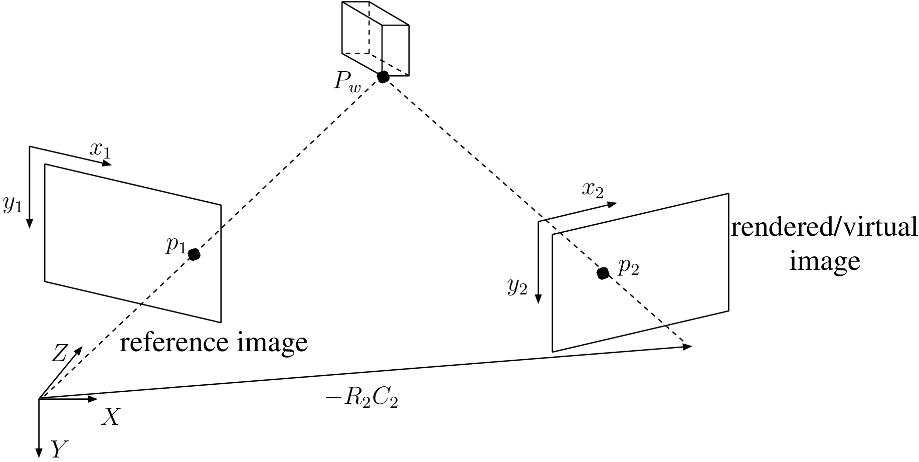
Figure 4.2 Two projection points \(\boldsymbol{p}_1\) and \(\boldsymbol{p}_2\) of a point \(\boldsymbol{P}_w\).

The orientation and location of the camera \(i\) (with \(i\in\{1,2\}\)) is described by the rotation matrix \(\boldsymbol{R}_i\) and translation matrix \(\boldsymbol{t}_i=-\boldsymbol{R}_i\boldsymbol{C}_i\), where \(\boldsymbol{C}_i\) describes the coordinates of the camera center. This allows us to define the pixel positions \(\boldsymbol{p}_1\) and \(\boldsymbol{p}_2\) in both image planes by

\[\begin{aligned} \lambda_1 \boldsymbol{p}_1 = \left[ \boldsymbol{K}_1 | \boldsymbol{0}_3 \right] \left[ \begin{array}{cc} \boldsymbol{R}_1 & \boldsymbol{-R}_1 \boldsymbol{C}_1 \\ \boldsymbol{0}_3^T & 1 \end{array} \right] \boldsymbol{P}_w = \boldsymbol{K}_1\boldsymbol{R}_1 \left( \begin{array}{c} X_w\\ Y_w\\ Z_w \end{array} \right) - \boldsymbol{K}_1\boldsymbol{R}_1 \boldsymbol{C}_1,\label{eq:left} (4.1) \\ \lambda_2 \boldsymbol{p}_2 = \left[ \boldsymbol{K}_2 | \boldsymbol{0}_3 \right] \left[ \begin{array}{cc} \boldsymbol{R}_2& \boldsymbol{-R}_2 \boldsymbol{C}_2 \\ \boldsymbol{0}_3^T & 1 \end{array} \right] \boldsymbol{P}_w = \boldsymbol{K}_2\boldsymbol{R}_2 \left( \begin{array}{c} X_w\\ Y_w\\ Z_w \end{array} \right) - \boldsymbol{K}_2\boldsymbol{R}_2 \boldsymbol{C}_2, \label{eq:right} (4.2) \end{aligned}\]

where \(\boldsymbol{K}_1\), \(\boldsymbol{K}_2\) represent the \(3 \times 3\) intrinsic parameter matrix of the corresponding cameras and \(\lambda_1\), \(\lambda_2\) are the homogeneous scaling factors. Assuming that the reference “Camera 1” is located at the coordinate-system origin (\(\boldsymbol{C}_1=\boldsymbol{0}_3\)) and looks along the \(Z\)-direction (\(\boldsymbol{R}_1=\boldsymbol{I}_{3 \times 3}\)), the scaling factor \(\lambda_1\) can be specified in this particular case by \(\lambda_1=Z_w\). From Equation (4.1), the 3D position of the original point \(\boldsymbol{P}_w\) in the Euclidean domain can be written as \[(X_w,Y_w,Z_w)^T=(\boldsymbol{K}_1\boldsymbol{R}_1)^{-1} \cdot ( \lambda_1 \boldsymbol{p}_1 + \boldsymbol{K}_1 \boldsymbol{R}_1 \boldsymbol{C}_1 ). (4.3) \label{eq:inv_p}\] Finally, we obtain the synthetic pixel position \(\boldsymbol{p}_2\) by substituting Equation (4.3) into Equation (4.2), so that \[\lambda_2 \boldsymbol{p}_2 = \boldsymbol{K}_2 \boldsymbol{R}_2( \boldsymbol{K}_1\boldsymbol{R}_1)^{-1}\cdot ( \lambda_1 \boldsymbol{p}_1 + \boldsymbol{K}_1 \boldsymbol{R}_1 \boldsymbol{C}_1 ) - \boldsymbol{K}_2 \boldsymbol{R}_2 \boldsymbol{C}_2. (4.4) \label{eq:warping}\] Assuming that “Camera 1” is located at the world coordinate system and looking in the \(Z\) direction, we rewrite the warping equation into \[\lambda_2 \boldsymbol{ p}_2 = \boldsymbol{ K}_2 \boldsymbol{R}_2 \boldsymbol{K}_1^{-1} Z_w \boldsymbol{p}_1 - \boldsymbol{K}_2 \boldsymbol{R}_2 \boldsymbol{C}_2. (4.5) \label{eq:warping_simple}\] Equation (4.5) constitutes the 3D image warping equation [66] that enables the synthesis of the virtual view from a reference texture view and a corresponding depth image.

One issue of the previously described method is that input pixels \(\boldsymbol{p}_1\) of the reference view are usually not mapped onto a point \(\boldsymbol{p}_2\) at integer pixel position. To obtain an integer pixel position, a simple heuristic technique is to map the sub-pixel coordinate \(\boldsymbol{p}_2\) to the nearest integer pixel position \(\hat{\boldsymbol{p}_2}\) with \(\hat{\boldsymbol{p}_2}=(\hat{y_2},\hat{x_2},1)=(\lfloor x_2+0.5 \rfloor, \lfloor y_2 +0.5 \rfloor,1)\). Additionally, to avoid undefined pixels in the rendered image, so-called pixel splat surfaces that cover multiple destination pixels, can be employed. In practice, a pixel splat simply enlarges the footprint of the destination pixel \(\boldsymbol{p}_2\), such that not only the color of \(\hat{\boldsymbol{p}_2}\) is defined but also some pixels surrounding \(\hat{\boldsymbol{p}_2}\). A second complication is that multiple original pixels can be projected onto the same pixel position in the virtual view. For example, a foreground pixel can occlude a background pixel in the rendered view, which results in overlapping pixels. Additionally, some regions in the virtual view are not visible from the original viewpoint, which results in holes in the virtual image (see Figure 4.3). The aforementioned issues are addressed with a rendering technique based on triangular meshes, which is presented in the next section.

Figure 4.3 A virtual view consists of visible, overlapped and undefined pixels.

Rendering using triangular meshes

To avoid rendering artifacts, a natural approach is to employ a mesh of triangles. The idea is to triangulate the reference depth image so that each triangle locally approximates the object surface. In our implementation, depth image triangulation is performed such that two micro-triangles per pixel are employed. For each triangle vertex in the reference image, the corresponding position of the warped vertex is calculated using Equation (4.4). Finally, a rasterization procedure is performed that converts the triangle-based geometric description of the warped image into a bitmap or raster image (see Figure 4.4). For an efficient implementation, it can be noticed that each adjacent triangle shares two common vertices. Therefore, only one warped-vertex position per pixel needs to be computed to obtain the third warped-vertex position.

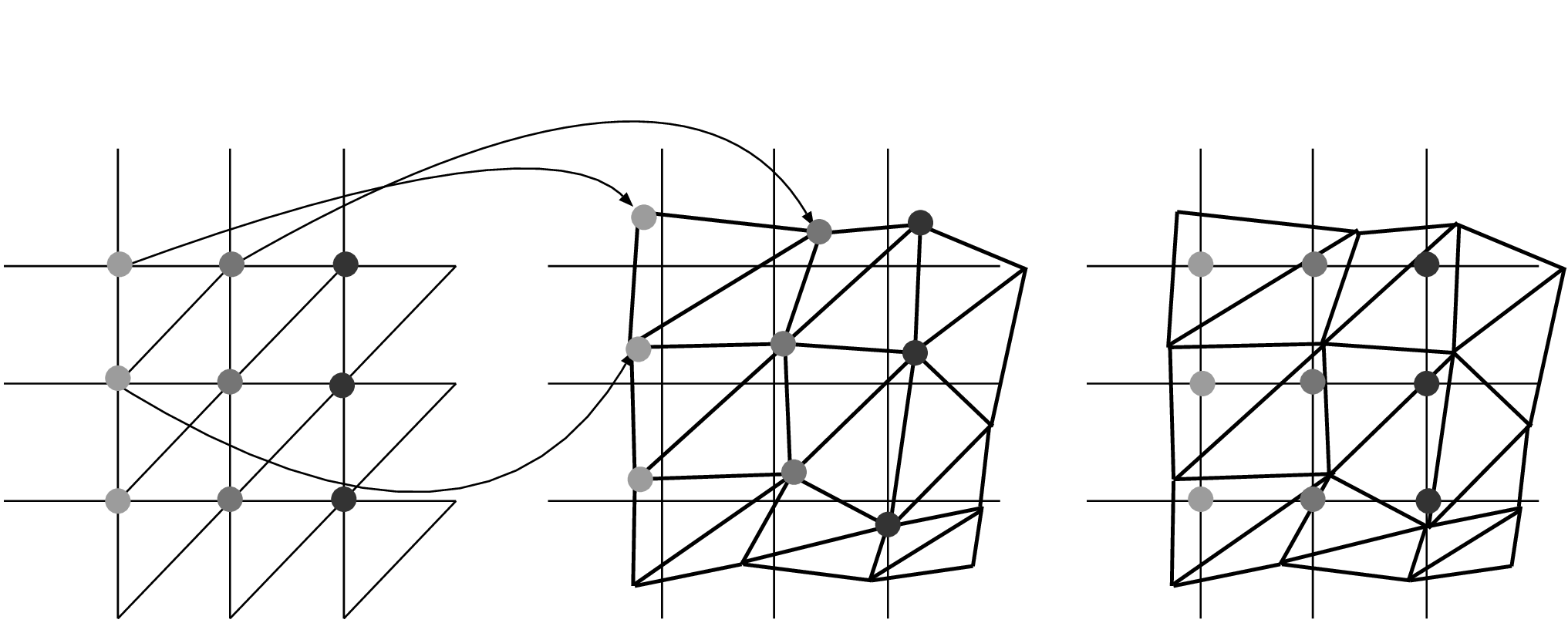
Figure 4.4 Stages of a micro-triangular mesh rendering technique: first, each triangle vertex in the reference image is warped and, second, each triangle is rasterized to produce the output image.

While such a technique leads to high-quality image rendering, a disadvantage is the very large number of micro-triangles, which involves a high computational complexity.

Rendering using relief texture mapping

As previously highlighted, the 3D image warping and the mesh-based rendering techniques suffer either from a low rendering quality, or a high computational complexity. To circumvent these issues, we now present an alternative rendering technique derived from the relief texture mapping algorithm [71]. Initially, relief texture mapping was developed for rendering uneven surfaces of synthetic computer graphics objects. The guiding principle of the relief texture mapping is to factorize the 3D image warping equation into a combination of simpler 2D texture mapping operations. In this section, we employ a similar approach, albeit adapted to the multi-view geometry framework.

Let us now factorize the warping function so that the equation is decomposed into a sequence of simple 2D texture mapping operations. From Equation (4.5), it can be written \[\frac{\lambda_2}{Z_w} \boldsymbol{p}_2 = \boldsymbol{K}_2 \boldsymbol{R}_2 \boldsymbol{K}_1^{-1} \cdot ( \boldsymbol{p}_1 - \frac{ \boldsymbol{K}_1 \boldsymbol{C}_2}{Z_w} ). (4.6) \label{eq:factor}\] Analyzing this factorized equation, it can be observed that the first factor \(\boldsymbol{K}_2 \boldsymbol{R}_2 \boldsymbol{K}_1^{-1}\) is equivalent to a \(3 \times 3\) matrix. This \(3 \times 3\) matrix corresponds to a homography transform between two images. In practice, a homography transform between two images is implemented using a planar texture mapping algorithm. The advantage of using such a transformation is that a hardware implementation of the function is available in a standard GPU.

Let us now analyze the second factor of the factorized equation, i.e., \( ( \boldsymbol{p}_1 - \frac{\boldsymbol{K}_1 \boldsymbol{C}_2}{Z_w} )\). This term projects the input pixel \(\boldsymbol{p}_1\) onto an intermediate point \(\boldsymbol{p}_i=(x_i,y_i,1)^T\), which can be defined as \[\lambda_i \boldsymbol{p}_i= \boldsymbol{p}_1 - \frac{\boldsymbol{K}_1 \boldsymbol{C}_2 }{Z_w}, (4.7) \label{eq:intermediate_image}\] where \(\lambda_i\) defines a homogeneous scaling factor. It can be seen that this last operation performs the translation of the reference pixel \(\boldsymbol{p}_1\) to the intermediate pixel \(\boldsymbol{p}_i\). The translation vector can be expressed in homogeneous coordinates by \[\lambda_i \left( \begin{array}{c} x_i \\ y_i \\ 1 \end{array} \right) = \left( \begin{array}{c} x_1 - t_1\\ y_1 - t_2\\ 1 - t_3 \end{array} \right) \textrm{, with } (t_1,t_2,t_3)^T=\frac{\boldsymbol{K}_1 \boldsymbol{C}_2 }{Z_w}. (4.8) \label{eq:pix_shift1}\] Written in Euclidean coordinates, the intermediate pixel position is defined by \[x_i= \frac{x_1-t_1}{1-t_3}, \qquad y_i= \frac{y_1-t_2}{1-t_3}. (4.9) \label{eq:pix_shift}\] It can be seen that the mapping from Equations (4.8) and (4.9) basically involves a 2D texture mapping operation, which can be further decomposed into a sequence of two 1D transformations. In practice, these two 1D transformations are performed first, along rows, and second, along columns. This class of warping methods is known as scanline algorithms [72]. An advantage of this supplementary decomposition is that a simpler 1D texture mapping algorithm can be employed (as opposed to 2D texture mapping algorithms). Hence, 1D pixel re-sampling can now be performed easily.

Let us now provide details about the pixel re-sampling procedure. Consider two consecutive pixels in the input reference depth image (see Figure 4.5). Following Equation (4.9), both pixels are first shifted horizontally in the intermediate image. Because both pixels are mapped onto sub-pixel positions, it is necessary to calculate and interpolate pixel values at integer pixel positions. A similar process is repeated column-wise to obtain the intermediate image.

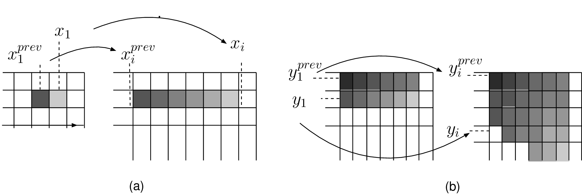
Figure 4.5 Two 1D pixel resampling operations. (a) In a first step, two consecutive pixels are horizontally shifted and re-sampled. (b) Next, re-sampled pixels are then projected onto the final intermediate image by performing vertical pixel shift followed by a pixel re-sampling procedure.

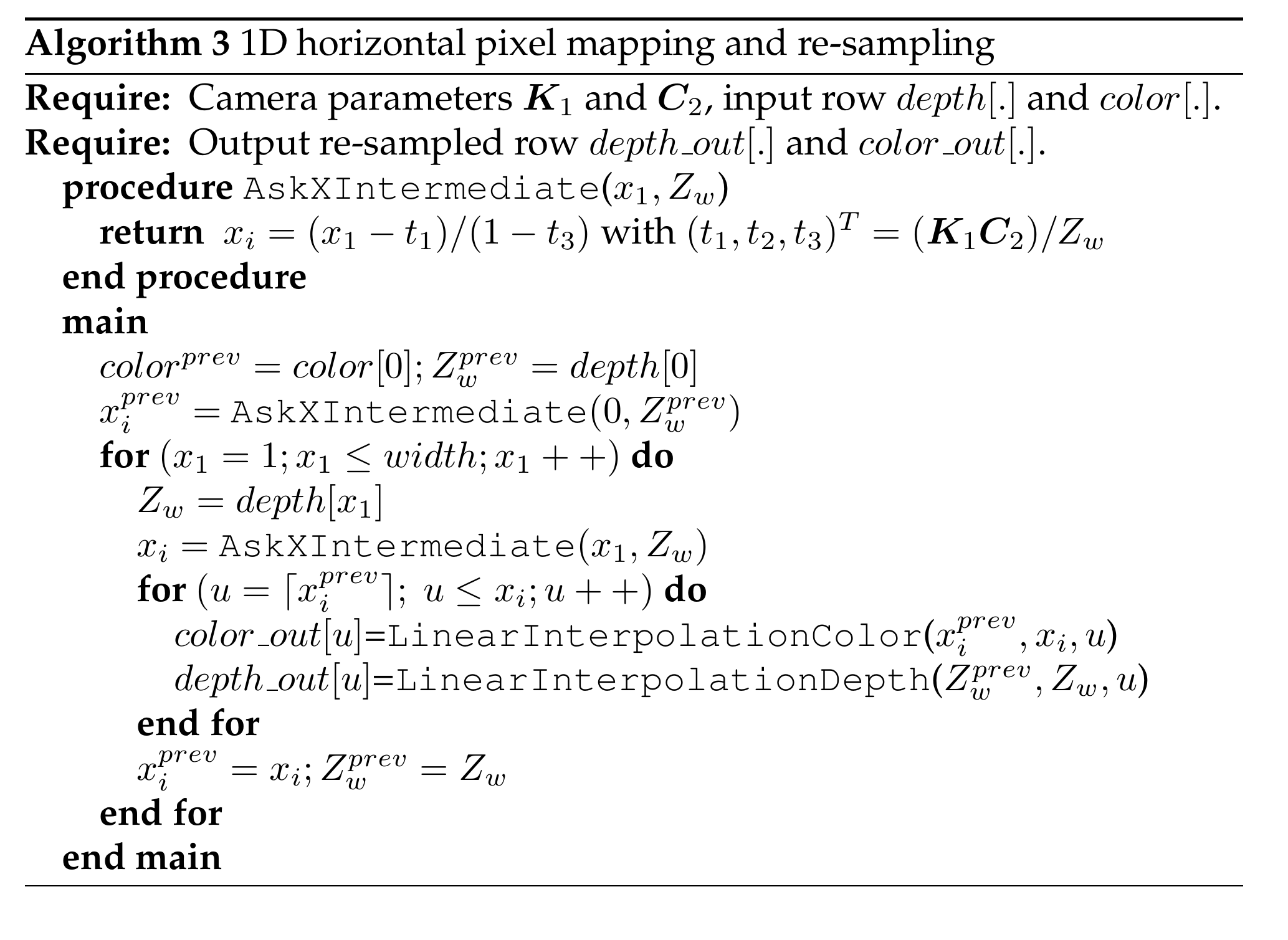
The pseudocode of the pixel re-sampling algorithm is summarized in Algorithm 3. In this pseudocode, the procedure LinearInterpolationColor(\(x_i^{prev},x_i,x\)) performs a linear interpolation between the \(color[x_i^{prev}]\) and \(color[x_i]\) at integer position \(x\). Similarly, the procedure LinearInterpolationDepth(\(x_i^{prev},x_i,x\)) performs a linear interpolation between \(depth[x_i^{prev}]\) and \(depth[x_i]\) at integer position \(x\).

The advantages of the relief texture algorithm are twofold. First, the described decomposition of the 3D image warping equation factorizes the equation into a sequence of two simpler 2D texture mapping operations. As a beneficial result, the implementation of the relief texture algorithm can be realized on a standard GPU, so that the rendering can be fastly executed. Second, the relief texture algorithm allows an accurate re-sampling of pixels, leading to an accurate rendering of fine textures. However, one disadvantage of the relief texture rendering technique is that the algorithm uses an intermediate image of arbitrary size, giving the algorithm an arbitrary computational complexity. More specifically, we have seen that the relief texture algorithm synthesizes an intermediate image (described by \(\boldsymbol{p}_i=\boldsymbol{p}_1- \frac{ \boldsymbol{K}_1 \boldsymbol{C}_2}{Z_w}\) in Equation (4.6)) prior to performing the planar texture mapping operation (described by \(\boldsymbol{K}_2 \boldsymbol{R}_2 \boldsymbol{K}_1^{-1}\) in Equation (4.6)). Because the intermediate pixel position \(\boldsymbol{p}_i\) depends on the arbitrary position of the virtual camera centered at \(\boldsymbol{C}_2\), the pixel \(\boldsymbol{p}_i\) may be projected in the intermediate image also at an arbitrary position. For example, intermediate pixels may be projected at negative pixel coordinates. A solution for handling intermediate pixels with negative coordinates consists is to use a large intermediate image of which the coordinate system is translated. Therefore, the relief texture algorithm requires an intermediate image of larger size. Practically, the size of the intermediate image is defined by calculating the position of the the four image corners for the minimum and maximum depth values (Equation (4.6).

Rendering using inverse mapping

A. Previous work

Let us now introduce an alternative technique to forward mapping, called inverse mapping. Prior to presenting the algorithm, we discuss the aspects of the earlier mentionned approaches and related work.

In the previous sections, three different image rendering algorithms were presented: 3D image warping, triangular mesh-based rendering and relief texture mapping. Each of these algorithms features some advantages and disadvantages. First, the 3D image warping provides a low complexity method for rendering images. However, the 3D image warping projects the source pixels onto the destination image grid at sub-pixel positions. As a result, the pixels in the synthetic image are not correctly re-sampled according to the integer pixel grid, resulting in re-sampling artifacts. Second, the triangular mesh-based rendering technique renders high-quality images at the expense of a high computational complexity. Finally, the proposed variant of the relief texture algorithm simultaneously features a high-quality rendering and a rendering-equation decomposition well suited for GPU architectures. However, the computational complexity varies with respect to the virtual camera position. Note that each of these rendering algorithms is defined as a mapping from the source image coordinates \(\boldsymbol{p}_1\) to the destination image coordinates \(\boldsymbol{p}_2\). Therefore, they are referred to as forward mapping. An alternative formulation is to define the rendering algorithm as a function of the destination image to the source image coordinates. Such a technique is usually referred to as inverse mapping. In particular, inverse mapping (back) projects destination pixels onto the source image grid. The color of the synthetic destination pixel is then interpolated from the pixels surrounding the calculated source pixel position. Therefore, the advantage of an inverse mapping rendering technique is that all pixels of the destination image are correctly defined and no holes can be distinguished in the rendered image. Figure 4.6 illustrates the image rendering process using inverse mapping.

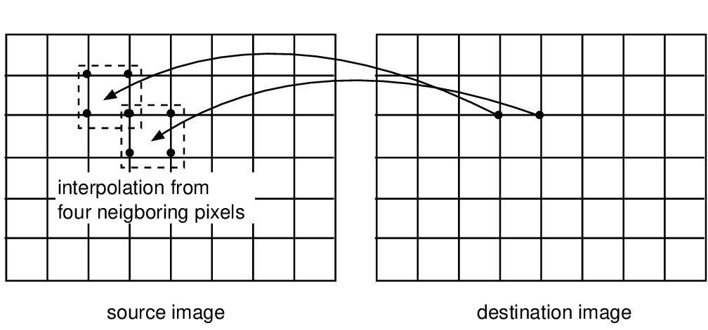
Figure 4.6 An inverse mapping function (back) projects a destination pixel onto the source image grid. The color of the destination pixel is then interpolated from the four neighboring pixels in the source image.

One of the earliest attempts for rendering images using inverse mapping, is based on a collection of uncalibrated and calibrated views [73]. The algorithm searches the color of the destination pixel that yields the most consistent color across the views. Using the geometry of multiple views, this is performed by searching the depth value of the destination pixel such that all pixel colors are consistent. This most consistent color is finally used as a color for the destination pixel. Because this method requires a search of depth values, the technique is computationally expensive. To avoid such an expensive search, the Sprite with Depth algorithm has been introduced [63]. The Sprite with Depth algorithm decomposes the source images into multiple planar sprite regions with known depth values and warps each sprite to the position of the destination image, thereby providing the per-pixel depth (in the destination image). As a result, an expensive search of depth is avoided. However, as mentioned in [63], because the source image is decomposed into multiple planar sprites, the Sprite with Depth algorithm can only handle 3D scenes with smoothly varying surfaces and short baseline distances between the cameras.

B. Rendering algorithm using inverse mapping

Bringing together ideas from both the Sprite with Depth algorithm and rendering from a collection of views, we propose an inverse mapping rendering algorithm that (a) allows a simple and accurate re-sampling of synthetic pixels, and (b) easily enables to combine multiple source images such that occluded regions can be correctly handled. It should be noted that property (a) is not fulfilled with the first presented 3D forward mapping algorithm, whereas the other two alternatives require complex re-sampling procedures. Property (b) is realized by scanning the interpolated view, so that the technique is forced to handle occluded regions by interpolating them from available views. The new algorithm can be summarized as follows.

Step 1: The depth map of the source image is warped at the position of the destination image (forward mapping of the depth image). This can be achieved using the 3D image warping equation (see Section 4.2.1), defined as \[\lambda_2 \boldsymbol{ d}_2 = \boldsymbol{ K}_2 \boldsymbol{R}_2 \boldsymbol{K}_1^{-1} Z_{1w} \boldsymbol{d}_1 - \boldsymbol{K}_2 \boldsymbol{R}_2 \cdot \boldsymbol{C}_2, (4.10) \label{eq:forward_mapping2}\] where \(\boldsymbol{d}_1\) and \(\boldsymbol{d}_2\) are depth pixel coordinates in the source and destination depth images, respectively, and \(\lambda_2\) a positive scaling factor. Thus, the depth value \(Z_{1w}\) is defined by the pixel value at coordinate \(\boldsymbol{d}_1\) in the source depth image. As defined in Section 4.2.1, \((\boldsymbol{K}_2,\boldsymbol{R}_2,\boldsymbol{C}_2)\) and \((\boldsymbol{K}_1)\) correspond to the camera parameters of the destination and source images, respectively. Note that the possible occluded holes are not padded in this stage.

Step 2: To avoid undefined pixels resulting from the forward mapping algorithm, a dilation operation is carried out on the rendered depth image. Next, two erosion operations which slightly reduce the delineation of foreground objects, are subsequently performed. This last step ensures that blended pixels at object borders are not classified as foreground pixels. Such a rendering artifact is described in detail in Section 4.4.1.

Step 3: Next, for each defined pixel \(\boldsymbol{d}_2\) of the destination depth image, a corresponding 3D world point \((X_{2w},Y_{2w},Z_{2w})^T\) is calculated using the back-projection operation defined by Equation (2.20) \[\left( \begin{array}{c} X_{2w}\\ Y_{2w}\\ Z_{2w} \end{array} \right) = \boldsymbol{C}_2+\lambda \boldsymbol{R}_2^{-1}\boldsymbol{K}_2^{-1}\boldsymbol{d}_2, (4.11)\] where \(\lambda\) is defined as \[\lambda=\frac{Z_{2w}-C_{2z}}{r_3} \textrm{ with } \left( \begin{array}{c} r_1\\ r_2\\ r_3 \end{array} \right) =\boldsymbol{R}_2^{-1}\boldsymbol{K}_2^{-1}\boldsymbol{d}_2 \textrm{ and } \boldsymbol{C}_2= \left( \begin{array}{c} C_{2x}\\ C_{2y}\\ C_{2z} \end{array} \right) . (4.12) \label{eq:backproj2}\] Here, the depth value \(Z_{2w}\) is defined by the pixel value at coordinate \(\boldsymbol{d}_2\) in the destination depth image. Thus, the depth value \(Z_{2w}\) is provided by the first step of the algorithm that warps the source depth image into the destination depth image.

Step 4: Finally, the calculated 3D point \((X_{2w},Y_{2w},Z_{2w})^T\) is projected onto the source texture image by employing \[\lambda \boldsymbol{p}_1 = \underbrace{ \left[\boldsymbol{K}_1 | \boldsymbol{0}_3\right] \left[ \begin{array}{cc} \boldsymbol{R}_1 & -\boldsymbol{R}_1\boldsymbol{C}_1 \\ \boldsymbol{0}_3^T & 1 \end{array} \right] } _{\textrm{projection matrix } \boldsymbol{M}_1} \left( \begin{array}{c} X_{2w}\\ Y_{2w}\\ Z_{2w}\\ 1 \end{array} \right), (4.13) \label{eq:projection_source_image}\] such that the color of the destination pixel \(\boldsymbol{p}_2\) can be interpolated from the pixels surrounding \(\boldsymbol{p}_1\) in the source image. The possible holes in the image are finally padded using a technique described in the following section.

The proposed inverse mapping rendering technique exhibits three advantages. First, because an inverse mapping procedure is employed, destination pixels can be accurately interpolated, thereby rendering high-quality virtual images. Second, we have seen that “Step 1” of the algorithm involves a forward mapping of the depth image. Intuitively, this processing step suffers from the usual problems associated with rendering using forward mapping. However, it should be noted that the depth image represents the surface of objects, so that the corresponding depth signal mainly features low-frequency components. As a result, forward-mapping depth images render images with limited rendering artifacts, when compared to rendered texture images. Third, the color of occluded pixels can be inferred at “Step 3” by projecting the 3D-world point \(\boldsymbol{p}_2=(X_{2w},Y_{2w},Z_{2w})^T\) onto multiple source image planes, covering all regions of the video scene. We describe this occlusion-handling scheme in detail in Section 4.4.3.

All rendering algorithms presented up to this point suffer from occlusion artifacts, such as creating holes that cannot reconstructed in the computed images, or overlapping pixels that cannot be interprated. This means that additional occlusion processing is required, which is presented in the following two sections.

Occlusion-compatible scanning order

This section presents a method that automatically prevents that background pixels overlap or hide the visibility of foreground pixels. Let us explain the overlapping problem in more detail. By construction, the presented rendering techniques define a mapping between source and destination pixels. However, one algorithmic issue is that multiple foreground and background source pixels can be mapped at the same position in the destination image. To determine the visibility of each pixel in the rendered view, a Z-buffer can be used that stores the depth of each pixel in the rendered view. When two pixels are warped at the same position, a depth comparison of the two pixels is performed and the foreground pixel with the smallest depth value is selected for rendering. However, this technique involves the usage of a memory buffer and a depth comparison for each warped pixel. An alternative technique is the occlusion-compatible scanning order [66] that we present in this section.

Occlusion-compatible scanning for rectified images

Let us first introduce the basic principle of the occlusion-compatible scanning order, using the simplified case of rectified images. To determine the visibility of each pixel in the rendered view, a practical method is to scan the original view such that eventually occluded background pixels are obtained prior to the occluding foreground pixels. Assuming that the views are rectified and that the intrinsic camera parameters are identical, the image rendering simply consists of a right-to-left pixel-shift operation, where the shift corresponds to the per-pixel disparity value [19]. Therefore, the rendering procedure is performed by scanning the disparity image in a left-to-right fashion such that foreground pixels overwrite background pixels, so that foreground pixels are always preserved. Additionally, to determine the positions of undefined pixels, a per-pixel flag is set when the interpolated pixel position is written. The collection of these per-pixel flags finally provides a map of occluded pixels. The procedure is illustrated by Figure 4.7.

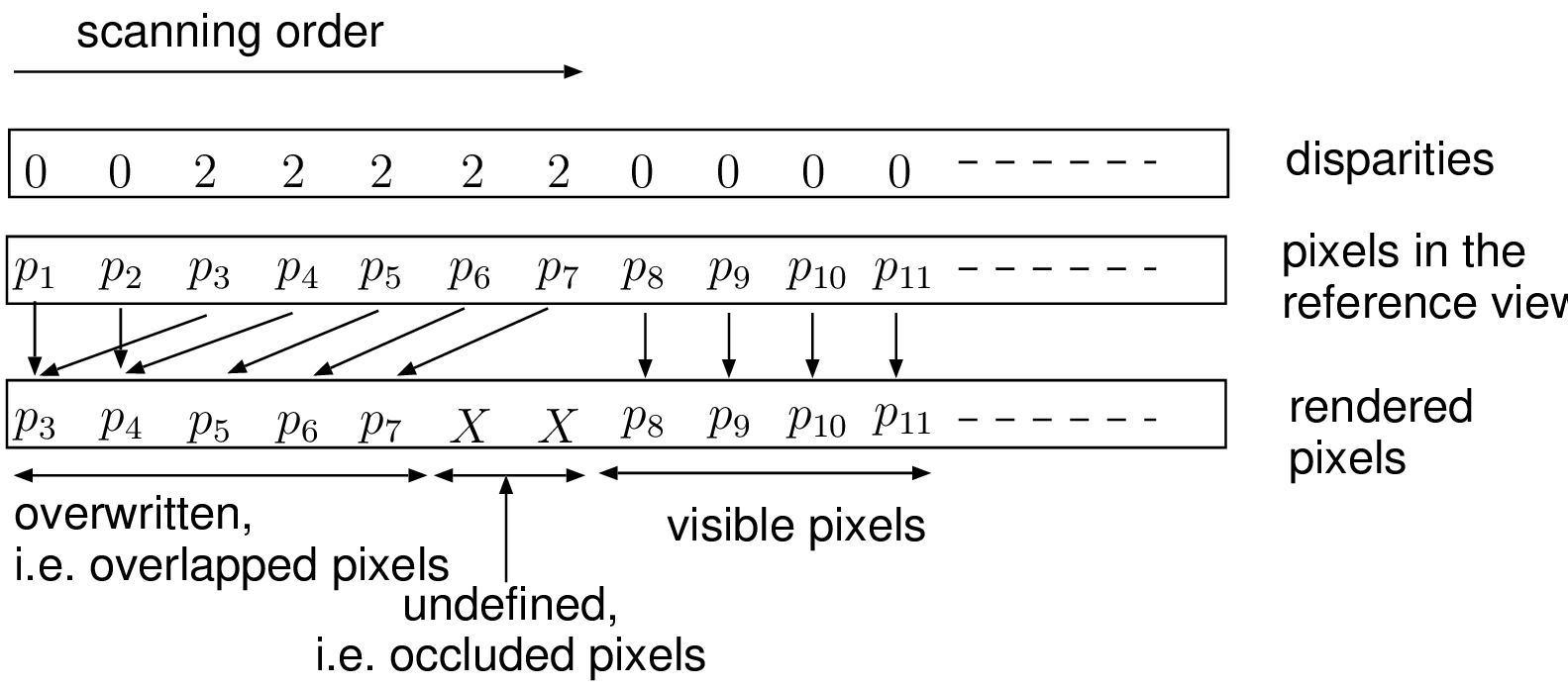
Figure 4.7 A proper scanning order of the original view enables that foreground pixels, \(p_3, p_4, p_5, p_6\) overwrite the background pixels, i.e., \(p_1\) and \(p_2\). Visible background pixels \(p_8, p_9, p_{10}, p_{11}\) are preserved. The arrows indicate a simple copy operation. The symbol \(X\) represents the occluded pixels.

Occlusion-compatible scanning for non-rectified images

The problem of scanning background pixels prior to foreground pixels using non-rectified images can be addressed using the occlusion-compatible scanning order [66]. Let us consider two 3D scene points \(\boldsymbol{P}_1\) and \(\boldsymbol{P}_2\), which are projected onto a target image (virtual view) at the same pixel position \(p\), and onto the reference view at pixel positions \(\boldsymbol{p}_1'\) and \(\boldsymbol{p}_2'\) (see Figure 4.8). To perform an occlusion-compatible scanning order of the reference image, it is necessary to scan first the 3D point \(\boldsymbol{P}_1\) and then \(\boldsymbol{P}_2\). Using the framework of oriented projective geometry [74], such a scanning can be obtained by considering the projection of the virtual/rendered camera center \(\boldsymbol{C}\) onto the reference image plane, i.e., the epipole \(\lambda_e'\boldsymbol{e'}=\boldsymbol{M'C}\). Specifically, two cases that depend on the sign of the scaling factor \(\lambda_e'\) can be distinguished.

• First, assuming \(\lambda_e'>0\), to perform the warping of background pixels \(\boldsymbol{p}_1\) prior to foreground pixels \(\boldsymbol{p}_2\), it is sufficient to scan the reference image from the border of the image towards the epipole \(e'\).

• Second, in the case \(\lambda_e'<0\), the reference image should be scanned from the epipole towards the borders of the image.

Whereas the first case follows from the discussion in Figure 4.7, the understanding of the second case is more complicated. We have worked on a proof of that case, for which a summary is presented in Appendix A.1.

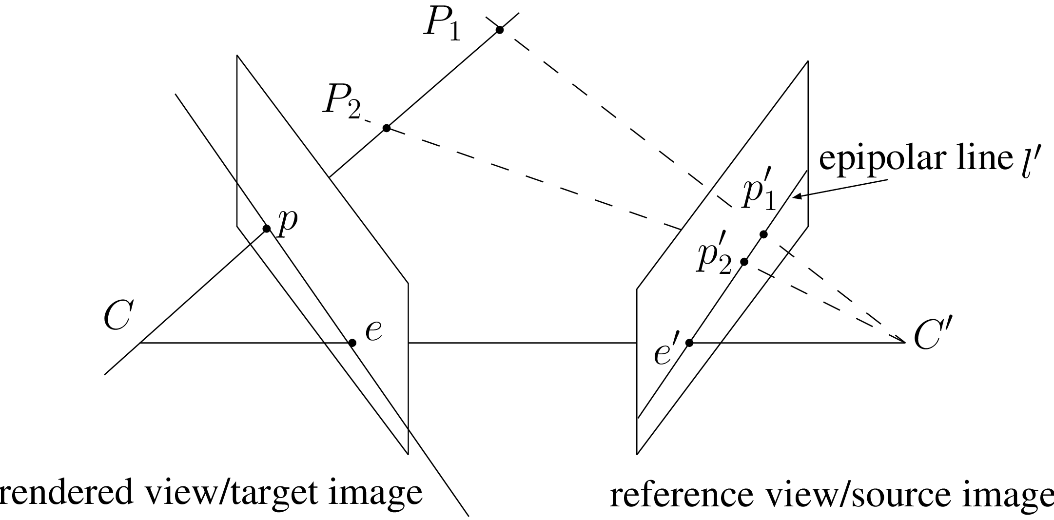
Figure 4.8 To perform the warping of background \(p_1'\) prior to foreground \(p_2'\), the reference image is scanned from the border toward the epipole \(e'\).

Occlusion handling

In the previous section, we have determined the scanning order of the reference image such that foreground objects overwrite background pixels. However, this still leaves open how the occluded pixels that may occur between foreground and background pixels should be interpolated. An illustration of undefined pixels noted as “X” is given in Figure 4.7. To interpolate these occluded pixels, we require a padding algorithm. In the sequel, we first present two conceptual algorithms based on the idea of scanning order and second, we propose an algorithm that resolves occlusions in a deterministic fashion.

Padding using occlusion-compatible scanning order

The first approach exploits the assumption that occluded pixels belong to the background. Therefore, an appropriate solution for padding occluded pixels is to fill undefined occluded regions by copying neighboring background pixels. To this end, the color of a neighboring background pixel should be determined. A proposal for doing this is to use the occlusion-compatible scanning order previously introduced in Section 4.3. The idea is to scan the destination image such that foreground pixels are scanned prior to background pixels. As a result, background pixels always overwrite occluded pixels. Note that, as opposed to the method presented in Section 4.3 for handling overlapping pixels, the original occlusion-compatible ordering algorithm scans the source image such that the background pixels are scanned prior to the foreground pixels. For holes, we thus scan in the opposite order. An example of a warped image with the occlusion padded with background pixels is shown in Figure 4.9(a).

(a)

(b) (c) (d) (e)

Figure 4.9 (a) Synthetic view using an occlusion-padding technique based on background pixels. (b) Magnified view that shows the “rubber band” effect. (c) Magnified view with stair-casing artifacts at the object boundaries. (d)+(e) Visual artifacts generated by propagating blended color in occluded pixels.

Unfortunately, as illustrated in Figure 4.9(b), because the padding is performed row by row, occluded regions show lines of equal pixels, which is called the “rubber band” artifact. Furthermore, in a typical textured image, object-border pixels show a mixture of foreground and background color, which results in blended color pixels. As a consequence, occluded pixels are padded by the blended color instead of the background color (see Figure 4.9(d) and Figure 4.9(e). To avoid the discussed artifacts, we have investigated an alternative padding technique that appropriately handles pixels at object boundaries.

Padding using occlusion-compatible scanning order and image pre-processing

As described previously, apparent artifacts mostly occur along object borders. Therefore, we now introduce a simple technique that intends to perform padding using non-blended pixels.

In a first step of the algorithm (image pre-processing), we replace the blended edge pixels in the original image. Because pixels along the object border are a mixture of foreground and background color, we classify the pixels on the object border as not valid (blended). To obtain the classification map of unreliable pixels, an edge-detection procedure is applied to the depth image. The algorithm then replaces each unreliable pixel by the nearest valid pixel in the image line. This results in an image in which object boundaries are not blended.

In a second step (padding), the non-blended image is warped and subsequently, edge pixels are blended. In this warping step, texture and depth samples are extrapolated from the background pixels (as described in the previous paragraph). Because the resulting warped view shows non-blended object boundaries, the algorithm finally smoothes the edges to obtain soft object boundaries. To attenuate the “rubber band” artifacts, the occluded regions are smoothened as well.

(a)

(b) (c) (d) (e)

Figure 4.10 (a) Synthetic view with occlusion padding based on background pixels and smoothened discontinuities. (b) “Rubber band” artifacts attenuated by smoothing the occluded pixels. (c) Attenuated stair-casing artifacts along the objects boundaries. (d) (e) Blended colors are not propagated in occluded pixels.

Though multiple heuristic techniques have been employed for padding the occluded pixels, experiments have revealed that the method can synthesize new views with sufficient quality for coding and visualization purposes. For example, Figure 4.10(d) and Figure 4.10(e) show that blended colors are not replicated in the occluded regions. Further objective rendering-quality measurements are presented in Section 4.5.

Occlusion handling using multiple source images

We now propose an occlusion-handling scheme that combines multiple source images such that all regions of the video scene are covered, i.e., not occluded. The proposed method is related to the work of [75], which also relies on multiple source images to correctly handle occluded pixels. The approach of [75] deals with occlusions by forward mapping two source images and compositing/blending the two warped images to obtain a single rendered destination image. However, it can be easily anticipated that this method entails the common problems associated with forward mapping of texture images. To address this problem, we build upon the inverse mapping rendering technique, as proposed in Section 4.2.4, and combine the inverse mapping technique with a multi-image rendering algorithm. The advantages of the proposed technique are twofold. First, it allows a simple and accurate re-sampling of synthetic pixels and, second, it easily combines multiple source images such that all regions of the scene are covered. Accordingly, the presented occlusion-handling technique heavily relies on the previously proposed inverse mapping rendering technique and can be described as follows.

Let us consider two source input texture images \(T_A\) and \(T_B\), combined with two depth images \(D_A\) and \(D_B\), and a destination texture image \(T_D\). Additionally, we associate a projection matrix \(\boldsymbol{M}^A_1\) and \(\boldsymbol{M}^B_1\) to each source texture image. The occlusion-rendering method can be divided into four steps.

Step 1: First, the two source depth images \(D_A\) and \(D_B\) are both warped at the position of the destination image using a forward mapping technique (see Equation (4.10)). Because a forward mapping rendering technique is used, both resulting warped depth images show holes, i.e., occluded pixels. Note that these holes are not padded. This enables the detection of occlusions at a later stage.

Step 2: To avoid undefined pixels resulting from the forward mapping algorithm, one dilation operation followed by two erosion operations are carried out on the rendered depth image (these choices were empirically determined). These undefined pixels do not refer to occluded regions, but to real undefined pixels that result from the forward mapping algorithm.

Step 3: Next, for each defined depth pixel, the coordinates of a 3D-world point are calculated using the back-projection Equation (2.20). We denote \(\boldsymbol{P}_2^A\) and \(\boldsymbol{P}_2^B\) as being the 3D-world points calculated using a depth pixel of the depth images \(D_A\) and \(D_B\), respectively. In the case that the depth pixel is undefined, the coordinates of the corresponding 3D-world point are set as undefined, accordingly.

Step 4: Finally, each defined 3D-world point is projected onto the source texture images \(T_A\) and \(T_B\), such that the source pixel coordinates \(\boldsymbol{p}_1^A\) and \(\boldsymbol{p}_1^B\) are obtained. More formally, this can be written as \[\lambda_1^A \boldsymbol{p}_1^A=\boldsymbol{M}_1^A \boldsymbol{P}_2^A \textrm{ and } \lambda_1^B \boldsymbol{p}_1^B=\boldsymbol{M}_1^B\boldsymbol{P}_2^B. (4.14)\] In the case that both source pixels \(\boldsymbol{p}_1^A\) and \(\boldsymbol{p}_1^B\) exhibit a consistent color, it can be inferred that the 3D point is visible in both source images, and the destination pixel can be defined as \(\boldsymbol{p}_1=(\boldsymbol{p}_1^A+\boldsymbol{p}_1^B)/2\). Alternatively, if both source pixels contain inconsistent colors, the foreground source pixel with the smallest depth value is selected to define the color of the destination pixel \(\boldsymbol{p}_1\). In practice, we have defined two pixels as consistent if their absolute difference is less than a specified threshold. In the case that both \(\boldsymbol{p}_1^A\) and \(\boldsymbol{p}_1^B\) are undefined, the pixels are padded using an occlusion-compatible scanning order that first scans the background objects prior to the foreground objects (Section 4.4.1).

The principal steps of the algorithm, as discussed and numbered above, are illustrated by Figure 4.11 for further clarification.

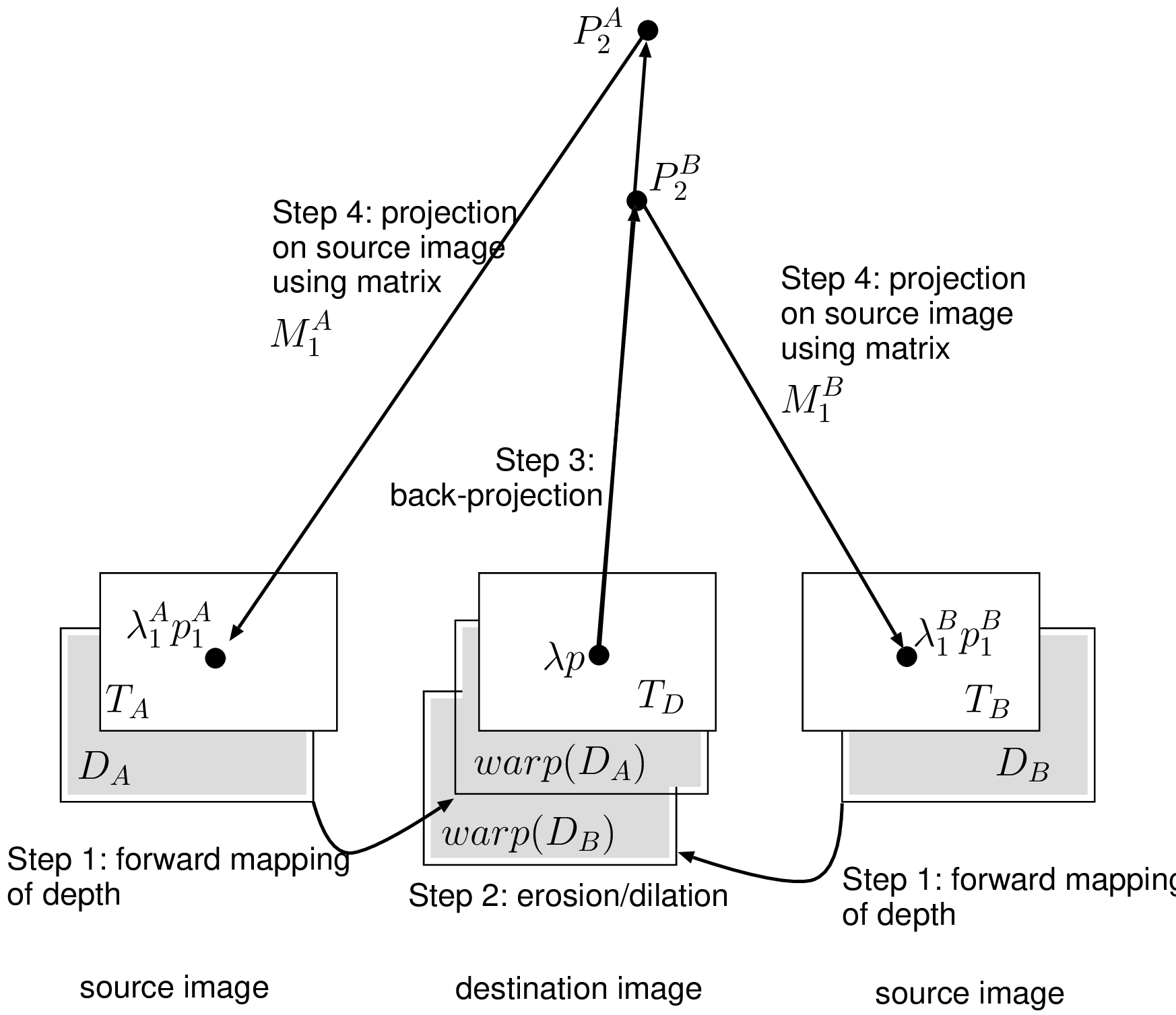
Figure 4.11 Occlusion handling using two source images \(T_A\) and \(T_B\) and the corresponding two depth images \(D_A\) and \(D_B\). In this example, the foreground 3D point \(\boldsymbol{P}_2^B\) occludes the background 3D point \(\boldsymbol{P}_2^A\). As a result, the color of the pixel \(\lambda \boldsymbol{p}\) is derived from the corresponding projected point \(\lambda_1^B \boldsymbol{p}_1^B\).

Experimental results on rendering quality and evaluation

This section evaluates various combinations of the algorithms presented in this chapter, ranging from rendering to padding and occlusion handling. In the experiments, we have explored the following image rendering algorithms: (1) 3D image warping, (2) mesh-based rendering algorithm, (3) relief texture mapping, (4) rendering using inverse mapping, and (5) rendering using inverse mapping of two source images.

To measure the quality of each rendering technique, a synthetic image is rendered at the same location and orientation of an arbitrarily selected camera (reference view). By comparing the synthetic and captured images, a distortion measure, e.g., \(\mathit{PSNR_{rs}}\) can be calculated. As defined in Chapter 3, the \(\mathit{PSNR_{rs}}\) distortion metric between a synthetic image \(I_s\) and a reference image \(I_r\) is calculated by \[\mathit{PSNR_{rs}} = 10 \cdot \log_{10} \left( \frac{255^2}{\mathit{MSE_{rs}}} \right), (4.15)\] where the Mean Squared Error (\(\mathit{MSE_{rs}}\)) is computed by the following equation: \[\mathit{MSE_{rs}} = \frac{1}{w \cdot h}\sum_{i=1}^{w}\sum_{j=1}^{h} ||I_r(i,j) - I_s(i,j)||^2, (4.16)\] with \(w\) and \(h\) corresponding to the width and the height of the image, respectively. For evaluating the performance of the rendering algorithms, experiments were carried out using the “Ballet” and “Breakdancers” texture and depth sequences (see Appendix A.2). Camera \(2\) was selected as a reference view while the Cameras \(1\) and \(3\) indicate the position and orientation of the rendered virtual views. The measured rendering qualities are summarized in Table 4.1. In the following discussion about the results of Table 4.1, the 3D image warping rendering is used as a reference for comparing results.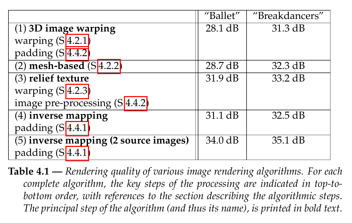

First, experiments have revealed that a mesh-based rendering method yields a rendering-quality improvement of 0.6 dB to 1.0 dB when compared with 3D image warping. This result demonstrates that a sub-pixel rendering algorithm is necessary to render high-quality images. However, we have found that this approach does not adequately handle occluded regions. Specifically, a mesh-based rendering method interpolates occluded pixels from the foreground and background pixels, so that occluded pixels are padded with a blend of foreground and background colors. Concluding, the gain of the mesh-based algorithm is deteriorated by an unappropriate handling of the occluded regions.

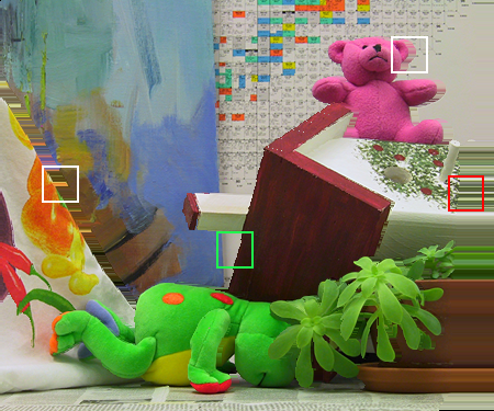
Next, we have compared the rendering quality of the relief texture mapping with the 3D image warping algorithm. Note that in this experiment, the source image is pre-processed using the technique described in Section 4.4.2 and that occluded pixels are padded using the color of the background pixels. Objective rendering-quality measurements show that padding of occluded pixels by the background color produces a noticeable improvement of the rendering quality. Specifically, we have obtained an image-quality improvement of \(1.9~dB\) and \(3.8~dB\), for the “Breakdancers” and “Ballet” sequences, respectively. Additionally, subjective evaluations demonstrate that the proposed rendering method enables high-quality rendered images. For example, the occluded regions at the right side of foreground characters are correctly extrapolated from the background color and any rendering artifacts are hardly perceived (see Figure 4.12(b) and Figure 4.14(b). This confirms that deriving the color of occluded regions from neighboring background pixels is a simple heuristic algorithm but an efficient approach.

Finally, the performances of two inverse mapping rendering techniques are evaluated. First, experimental results show that the inverse mapping rendering technique improves the rendering quality up to 3 dB, when compared to 3D image warping. In addition, it can be noted that the relief texture rendering method slightly outperforms the inverse mapping rendering technique. Such a result simply emphasizes that the occlusion-handling technique has a significant impact on the final rendering quality. In this specific case, the occlusion-handling technique, which includes the image pre-processing step, produces significant rendering improvements (see Figure 4.13(a) and Figure 4.15(a)).

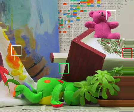
Second, the two-image inverse mapping technique is compared with the 3D image warping algorithm. Objective rendering-quality measurements show that a significant rendering-quality improvement can be obtained by combining two source images for synthesizing a single image. For example, an improvement of 3.8 dB and 5.9 dB is obtained for the “Breakdancers” and “Ballet” sequences, respectively. Additionally, subjective evaluations show that occluded regions are adequately handled. For example, the occluded regions at the right of the foreground persons in Figure 4.13(b) and Figure 4.15(b) are correctly defined and rendered accurately. Note that, as opposed to the heuristic padding technique, the occluded region is now correctly defined.

For comparison purposes, we have developed a C++ software implementation of the rendering algorithms. Since the presented work focuses on the quality of the rendered images, the software implementation was not optimized for fast rendering. Practically, our software implementation yields a rendering time that ranges between 3.5 and 7 seconds for each frame (of size \(1024\times 768\) pixels). Again, note that this rendering time is not obtained from an optimized software implementation. It is thus possible to significantly reduce the rendering time by using a Single Instructions Multiple Data (SIMD) processor architecture, which is available in modern CPU’s. Considering a possible GPU-based optimization of the relief texture mapping algorithm, we have found that using a GPU-based acceleration does not bring execution performance improvements. Specifically, although the execution of the homography transform is performed efficiently by the GPU, the speed for transferring the resulting synthetic image from the graphic GPU memory to the main CPU memory is low, so that not computation but bandwidth is the bottleneck. Currently, this communication bottleneck has been addressed by the latest generation of modern GPU’s.

Conclusions

In this chapter, we have proposed two novel image rendering algorithms.

The first algorithm is based on a variant of the relief texture method. As opposed to the original approach adapted to a computer-graphics framework, the proposed algorithm directly integrates the internal and external camera parameters. To enable accurate rendering, the proposed rendering algorithm decomposes the standard image warping equation into a sequence of two simpler 2D operations. The first 2D operation is further decomposed into two 1D operations, thereby enabling a simple re-sampling of pixels along rows and columns. The second 2D operation is an homography transform that can be accurately implemented and efficiently executed using a standard GPU. As a result, the key features of the algorithm are that it avoids holes in the synthetic image and it fits well to a GPU architecture.

The second algorithm is based on an inverse mapping method that scans the destination image and calculates the position of the corresponding pixels in the source image. Therefore, this methods allows a simple re-sampling of synthetic pixels because it prevents rounding the coordinates of synthetic pixels to the underlying pixel grid. The proposed rendering algorithm features a simple and accurate re-sampling of synthetic pixels and easily enables the combination of multiple source images such that occluded regions can be correctly handled. Therefore, this algorithm can potentially offer a higher rendering quality than the relief texture mapping.

Next, to address the problem of determining the visibility of background and foreground pixels in the rendered image, we have discussed the occlusion-compatible scanning order. This concept was adopted from literature and validated within our framework. Here, we have derived that a proper scanning can be made for rectified and unrectified views.

Additionally, two occlusion-handling techniques were introduced. The first technique is based on the assumption that occluded regions correspond to background pixels. Occluded pixels are therefore padded using the color of neighboring background pixels. Although the presented techniques are based on heuristic rules, experimental results have shown that the relief texture combined with the proposed occlusion-handling methods yield between 1.9 dB and 3.8 dB rendering-quality improvement. The second occlusion-handling method combines two source images that cover all regions of the video scene for synthesizing a single virtual view. Note that the proposed inverse mapping algorithm integrates and combines the two source images by careful pixel selection, so that occluded regions are properly handled. Experimental results indicate that such an occlusion-handling technique further improves the rendering quality by a range of 3.8 dB to 5.9 dB.

If there is one aspect of this chapter that comes clearly to the foreground, then it is a decent solution for the occlusion problem. If this is well managed, the rendering quality will be clearly improved, both objectively in terms of measured SNR (dB) and subjectively. It will become clear later in this thesis, that this also has a beneficial impact on the coding efficiency, since the visual data contains less disturbing and noisy pixels. A second aspect is that an efficient use of the multi-view geometry can significantly reduce the complexity of the rendering algorithms. Specifically, we have seen that the visibility of objects can be determined by solely using the multi-view geometry without any depth information. Additionally, the multi-view geometry enables an efficient and simple padding of background holes in the synthetic images. Finally, we have seen that a rendering equation relying on the multi-view geometry can be appropriately factorized, thereby enabling an efficient execution. The aforementioned advantages highlight that multi-view geometry constitutes a very powerful tool ¹¹, which was indispensable in this chapter for making the improvements and optimizations with a limited number of assumptions and conditions.

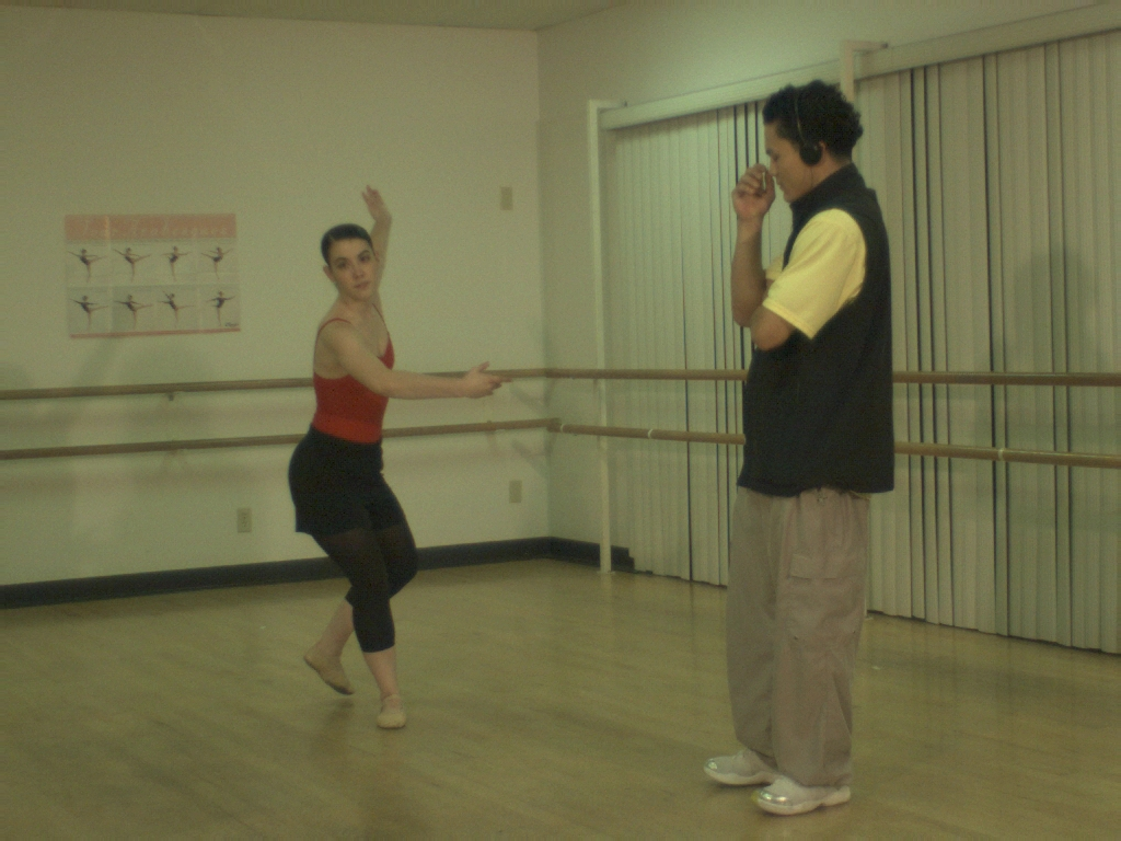
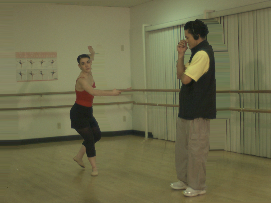
Figure 4.12 (a) Original view of the “Ballet” sequence captured by the camera 3. (b) Relief texture mapping algorithm.

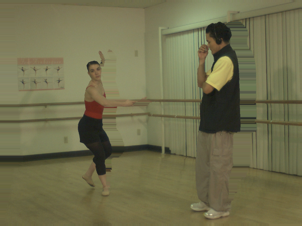
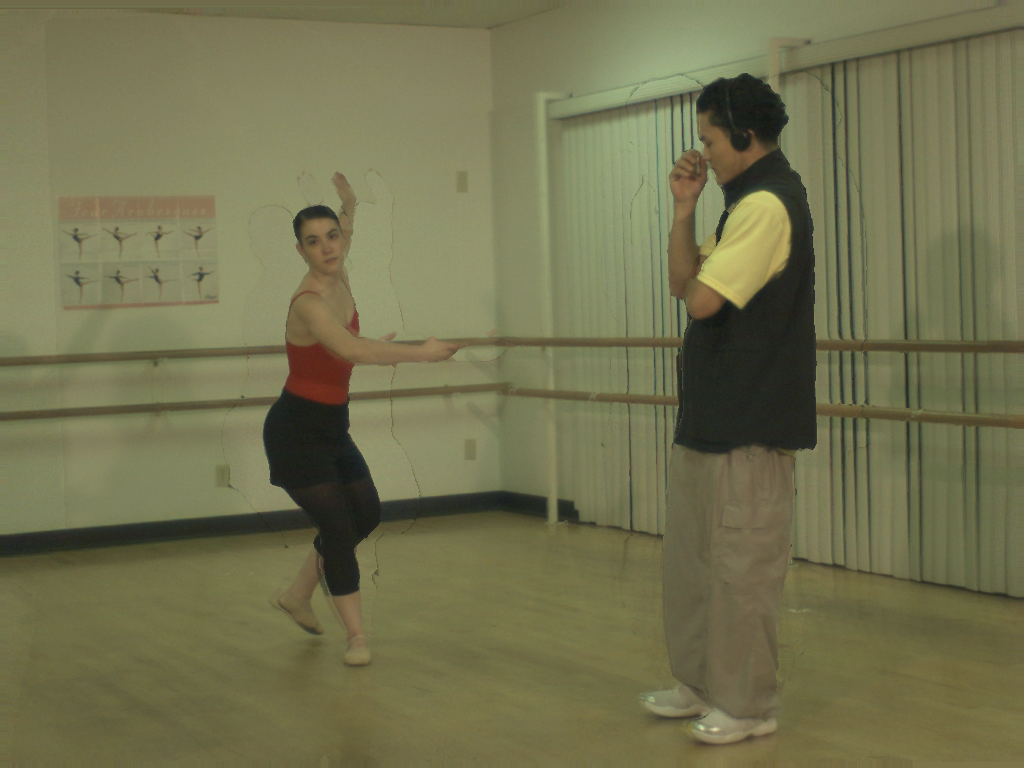
Figure 4.13 (a) Inverse-mapping algorithm. (b) Inverse-mapping algorithm using two source images.

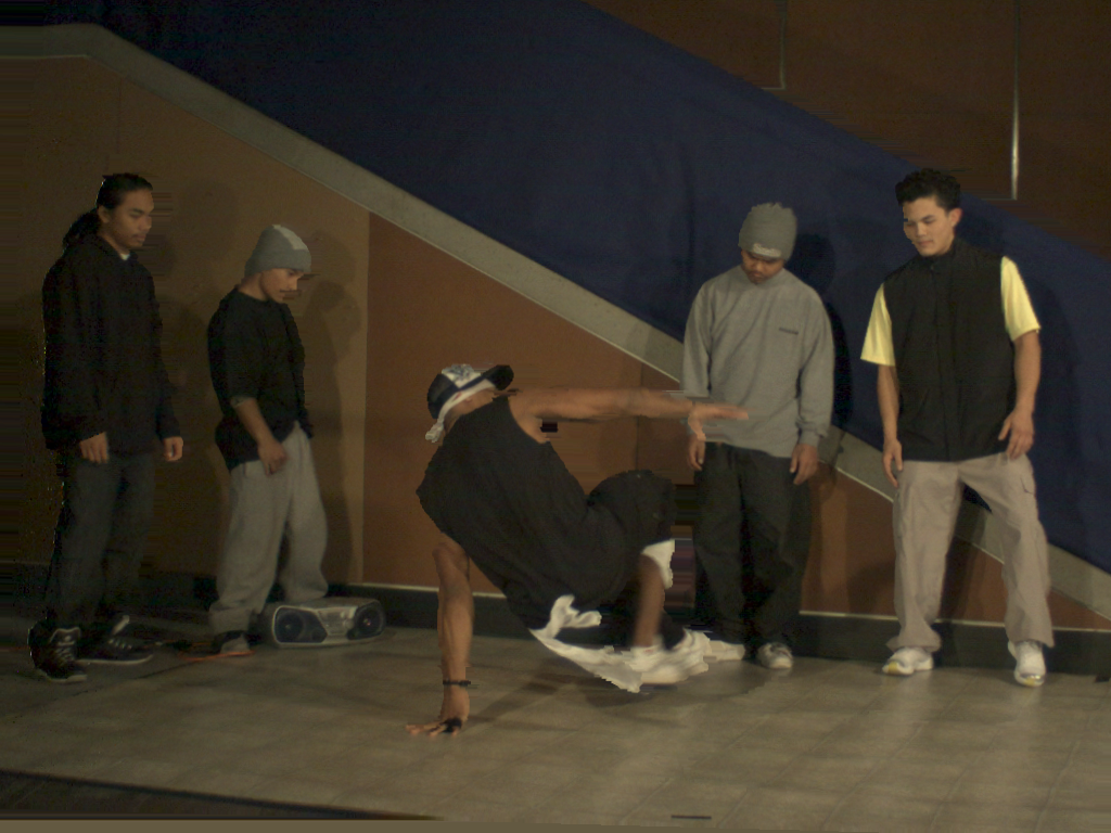
Figure 4.14 (a) Original view of the “Breakdancers” sequence captured by the camera 3. (b) Relief texture mapping algorithm.

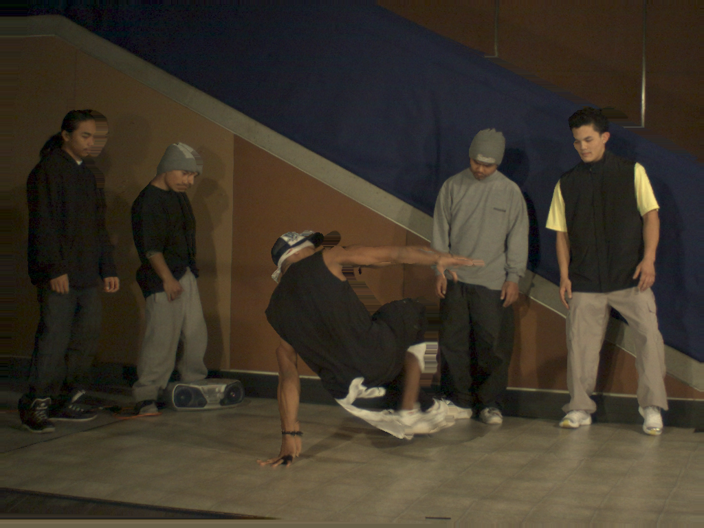
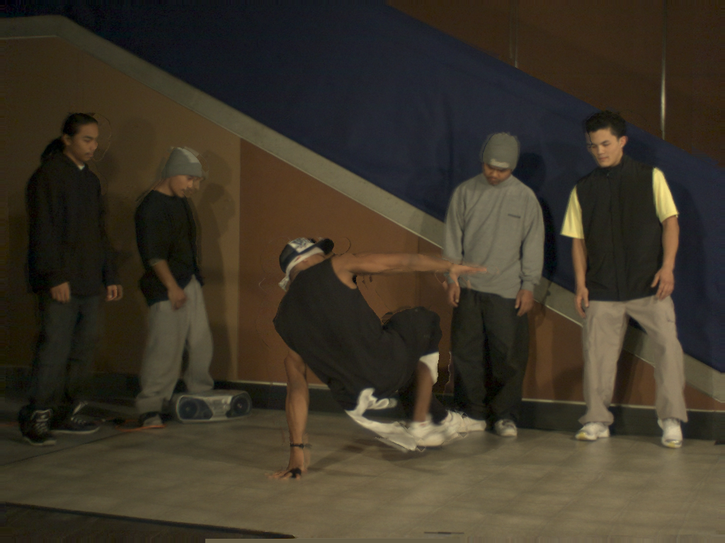
Figure 4.15 (a) Inverse-mapping algorithm. (b) Inverse-mapping algorithm using two source images.

Reference