Multi-View Depth Estimation

This chapter describes algorithms for estimating the depth of pixels, based on the projective geometry framework introduced in the previous chapter. In the first part, we focus on the estimation of depth images using two views. The key is a description of the basic geometric model and an elementary method that is employed to triangulate the depth of points from two (rectified) images. Because this elementary method results in an inaccurate depth estimation, we subsequently review two depth-calculation/optimization strategies: a local and a one-dimensional optimization strategy. In the second part of this chapter, we show that, instead of employing only two rectified views, multiple views can be employed simultaneously to estimate the depth. Based on this observation, we propose a multi-view depth estimation technique that (1) increases the smoothness properties of estimated depth images, and (2) enforces consistent depth images across the views.

Introduction

In the previous chapter, we have introduced the fundamentals of multi-view geometry that model the projection of a 3D point onto the 2D image plane. In this chapter, we employ the geometry of multiple views to solve the inverse problem of estimating the 3D position (depth) of a point using multiple 2D images.

Depth estimation aims at calculating the structure and depth of objects in a scene from a set of multiple views or images. The problem is to localize corresponding pixels in the multiple views, i.e., point-correspondences, that identify the same 3D scene point. By finding those point-correspondences, the depth information can be derived by triangulation. In the case point-correspondences are estimated for each non-occluded pixel, a so-called dense depth map or depth image can be constructed (see Figure 3.1).

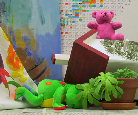
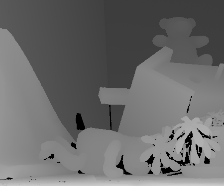
Figure 3.1 The depth of a pixel can be derived by triangulating multiple views of the scene (here, two views (a) and (b)). (c) The scene structure represented in a so-called depth image.

One important application of depth maps is image rendering for free-viewpoint video and 3D-TV systems. For such applications, we have seen in Section 1.3 that a 3D video scene can be represented efficiently by using one depth image for each texture view. In such a case, multi-view depth images should be computed or estimated. We define multi-view depth images as a set of depth images corresponding to the multiple captured texture views. Considering the multi-view video acquisition and compression framework, the multi-view depth images should:

• be accurately estimated so that high-quality images can be rendered,

• present smooth properties on the object surfaces so that a high compression ratio (of depth images) can be obtained,

• have sharp discontinuities along object borders so that a high rendering quality can be obtained,

• be consistent across the views so that the multi-view compression system can exploit the inter-view redundancy (between depth views).

At first glance, the second and third objective may look contradictory, but the reader should consider that properties of surfaces are different from the properties of the borders of an object. The proposed depth estimation algorithm handles this difference by adapting the smoothness requirement at object borders, i.e., depth discontinuities.

In the first part of this chapter, we focus on the problem of estimating the depth using two views. To simplify the understanding of the problem, the restricted case of depth estimation using two rectified views is considered. Assuming this restricted case, we present an elementary depth image estimation algorithm and discuss corresponding difficulties. To calculate more accurate depth estimates, we review two optimization strategies: a local and a one-dimensional optimization technique. Results when using these two techniques showing estimated depth images and intermediate conclusions are presented.

In the second part, we extend the two-view depth-estimation algorithm to the case of multiple views. Based on this extension, we propose two new constraints that enforce consistent depth estimates across the scanlines (inter-line smoothness constraint) and across the views (inter-view smoothness constraint). We show that these additional constraints can be readily integrated into the optimization algorithm and significantly increase the accuracy of depth estimates. As a result, both constraints yield smooth and consistent depth images across the views, so that a high compression ratio can be obtained.

Two-view depth estimation

Two-view geometry

We now describe the geometry that defines the relationship between two corresponding pixels and the depth of a 3D point. Let us consider a 3D Euclidean point \((X,Y,Z)^T\) captured by two cameras and the two corresponding projected pixels \(\boldsymbol{p}_1\) and \(\boldsymbol{p}_2\). Using the camera parameters (see Equation (2.18)), the pixel positions \(\boldsymbol{p}_1=(x_1,y_1,1)^T\) and \(\boldsymbol{p}_2=(x_2,y_2,1)^T\) can be written as \[\lambda_i \boldsymbol{p}_i = \boldsymbol{K}_i\boldsymbol{R}_i \left( \begin{array}{c} X\\ Y\\ Z \end{array} \right) - \boldsymbol{K}_i\boldsymbol{R}_i \boldsymbol{C}_i \textrm{ with } i\in\{1,2\}. (3.1)\]

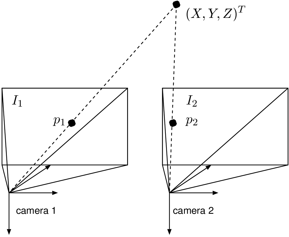
Figure 3.2 Two aligned cameras capturing rectified images can be employed to perform the estimation of the depth using triangulation.

The previous relation can be simplified by considering the restricted case of two rectified views so that the following assumptions can be made. First, without loss of generality, the world coordinate system is selected such that it coincides with the coordinate system of camera 1 (see Figure 3.2). In such a case, it can be deduced that \(\boldsymbol{C}_1=\boldsymbol{0}_3\) and \(\boldsymbol{R}_1=\boldsymbol{I}_{3 \times 3}\). Second, because images are rectified, both rotation matrices are equal: \(\boldsymbol{R}_1=\boldsymbol{R}_2=\boldsymbol{I}_{3 \times 3}\). Third, camera \(2\) is located on the \(X\) axis: \(\boldsymbol{C}_2=(t_{x_2},0,0)\). Finally, and fourth, both cameras are identical, so that the internal camera parameter matrices are equal, leading to \[\boldsymbol{K}=\boldsymbol{K}_1=\boldsymbol{K}_2= \left( \begin{array}{ccc} f&0 &o_x\\ 0&f &o_y\\ 0&0 & 1\\ \end{array} \right). (3.2)\] Equation (3.1) can now be rewritten as \[\lambda_1 \left( \begin{array}{c} x_1\\ y_1\\ 1 \end{array} \right) = \boldsymbol{K} \left( \begin{array}{c} X\\ Y\\ Z \end{array} \right) \textrm{ and } \lambda_2 \left( \begin{array}{c} x_2\\ y_2\\ 1 \end{array} \right) = \boldsymbol{K} \left( \begin{array}{c} X\\ Y\\ Z \end{array} \right) - \boldsymbol{K} \left( \begin{array}{c} t_{x_2}\\ 0\\ 0 \end{array} \right) . (3.3)\] By combining both previous relations, it can be derived that \[\left( \begin{array}{c} x_2\\ y_2 \end{array} \right) = \left( \begin{array}{c} x_1-\frac{f \cdot t_{x_2}}{Z}\\ y_1 \end{array} \right) . (3.4)\] Equation (3.4) provides the relationship between two corresponding pixels and the depth \(Z\) of the 3D point (for the simplified case of two rectified views). The quantity \(f \cdot t_{x_2} / Z\) is typically called the disparity. Practically, the disparity quantity corresponds to the parallax motion of objects ⁶. The parallax motion is the motion of objects that are observed from a moving viewpoint. This can be illustrated by taking the example of a viewer who is sitting in a moving train. In this example, the motion parallax of the foreground grass along the train tracks is higher than a tree far away in the background.

It can be noted that the disparity is inversely proportional to the depth, so that a small disparity value corresponds to a large depth distance. To emphasize the difference between both quantities, we indicate that the following two terms will be used distinctively in this thesis.

• Disparity image/map: an image that stores the disparity values of all pixels.

• Depth image/map: an image that represents the depth of all pixels.

The reason that we emphasize the difference so explicitly, is that we are going to exploit this difference in the sequel of this thesis. Typically, a depth image is estimated by first calculating a disparity image using two rectified images and afterwards, by converting this disparity into depth values. In the second part of this chapter, we show that such a two-stage computation can be circumvented by directly estimating the depth using an alternative technique based on an appropriate geometric formulation of the framework.

Simple depth estimation algorithm

Based on the previously described geometric model, a simple depth estimation algorithm can be detailed as follows. Let us consider a left- and right-rectified image denoted by \(I_1\) and \(I_2\), respectively. To perform depth estimation, it is necessary to establish the point-correspondence \((\boldsymbol{p}_1,\boldsymbol{p}_2)\) for each pixel. Selecting the pixel \(\boldsymbol{p}_1\) as a reference, a simple strategy consists of searching for the pixel \(\boldsymbol{p}_2\) that corresponds to pixel \(\boldsymbol{p}_1\) along the epipolar line. Because the images are rectified, we search for the point-correspondence along horizontal raster scanlines. To limit the search area, a maximum disparity value \(d_{max}\) is defined. The similarity between pixels \(\boldsymbol{p}_1\) and \(\boldsymbol{p}_2\) is measured using a matching block (window) \(W\) surrounding the pixels (see Figure 3.3).

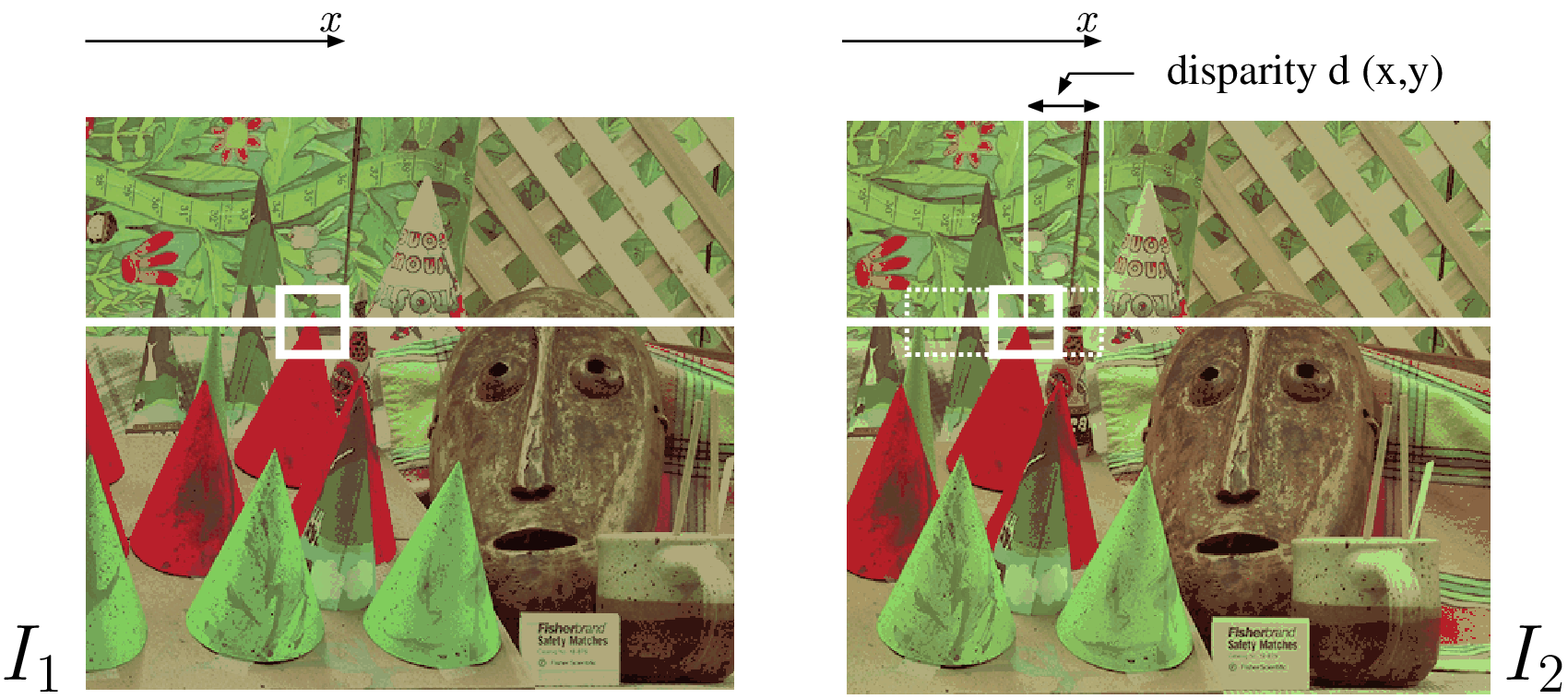
Figure 3.3 The disparity is estimated by searching the most similar block in the second image \(I_2\) along a one-dimensional horizontal epipolar line.

Employing the Sum of Absolute Differences (SAD) as a similarity measure for block comparison, the disparity \(d\) of a pixel at position \((x,y)\) in view \(I_1\) can be written as \[d(x,y)={\mathop{\textrm arg\, min}}_{0\leq \tilde{d}\leq d_{max}} \sum_{(i,j)\in W} | I_1(x+i,y+j)-I_2(x+i-\tilde{d},y+j)|. (3.5)\] The previous operation is repeated for each pixel so that a dense disparity map is obtained. To convert the obtained disparity map into a depth image, Equation (3.4) should be employed. Because the technique relies on a block-matching procedure, the attractiveness of the approach is its computational simplicity. However, this simple technique results in inaccurately estimated disparity values. For example, a change of illumination across the views introduces ambigpuities. Besides this, other difficulties arise that we now discuss in more detail.

Difficulties of the described model

The calculation of depth using point-correspondences is an ill-posed problem in many situations, which are summarized below.

D1: Texture-less regions. To estimate the disparity, a similarity or correlation measure is employed. However, in the case the disparity is estimated over a region of constant color, the correlation function yields a constant correlation/matching score for all disparity values. Therefore, all disparity values yield an equal correlation measure. Practically, this results in unreliable disparity estimates.

D2: Occluded regions. As illustrated by Figure 3.4, regions in the scene may not be visible from the two selected viewpoints, called occluded regions. In this case, because it is not possible to detect point-correspon-dences from occluded regions, no depth information can be calculated.

D3: Contrast changes across the views. When capturing two images with two different cameras, the contrast settings and illumination may differ. This results in different intensity levels across the views yielding unreliable matches.

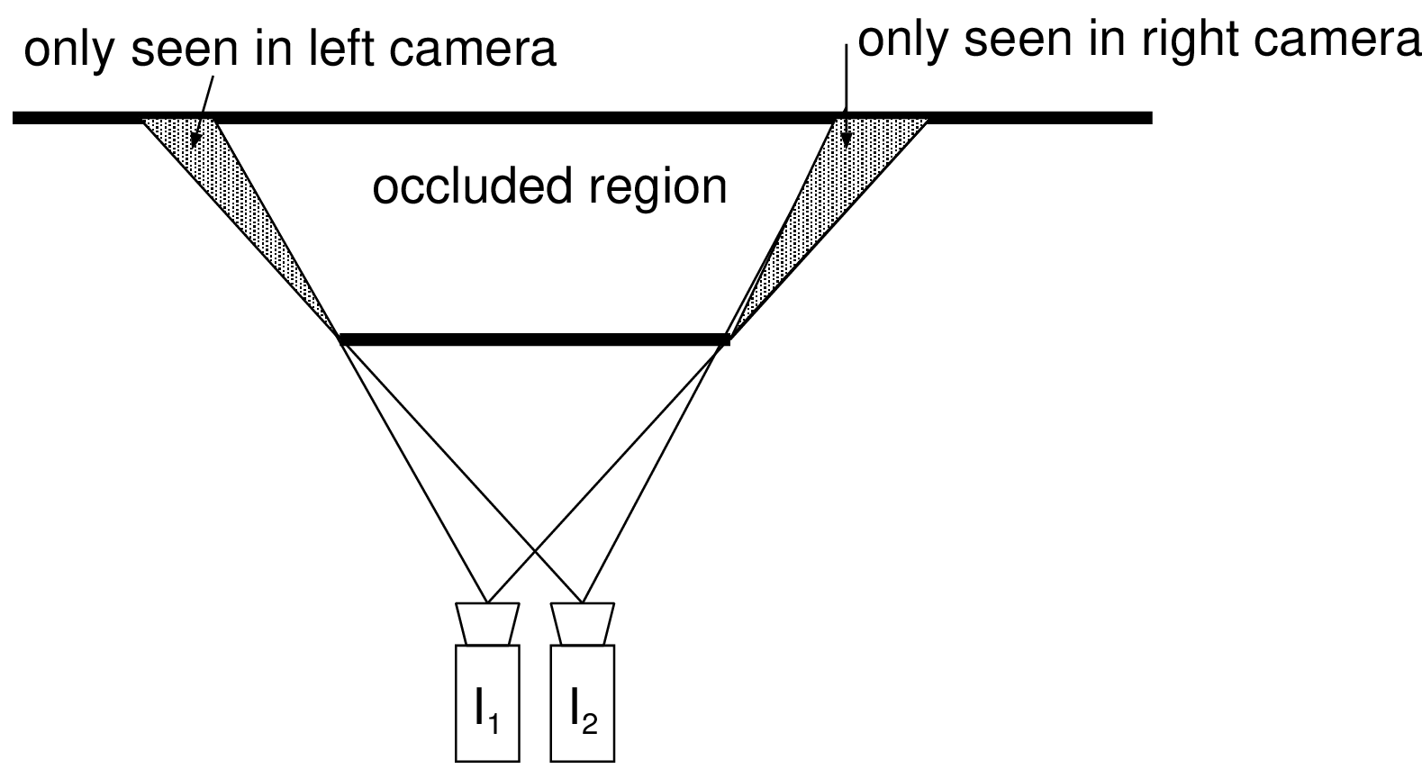Figure 3.4 Some regions visible in the image \(I_1\) are occluded in the image \(I_2\), which blocks the detection of point-correspondences.

To address the previously discussed issues, we now review previous work on depth estimation from literature.

Previous work on depth estimation

The problem of depth estimation has been intensively investigated in the computer-vision research community [37]. The author distinguishes three essential components, constituting most of the depth-estimation algorithms: (1) the matching criterion or cost function, (2) the support of the matching function and (3) the disparity calculation/optimization strategy.

Matching criterion

The first elementary component corresponds to the matching criterion that measures correlation or similarity between pixels. These include, among others, the Sum of Absolute Differences (SAD), the Sum of Squared Differences (SSD), the Cross Correlation (CC), and the Normalized Cross-Correlation (NCC). However, as highlighted in the literature [38], the selection of the matching cost function does not have a significant impact on the quality of the correspondence matching. We employ in our experiments the Sum of Absolute Differences (SAD) as a matching cost function. This SAD metric is calculated for the three color channels and the resulting three SAD values are simply added. However, it is known [38] that the three color channels are correlated, so that employing three color channels does not triple the matching accuracy. Thus, using the three color channels (instead of one luminance channel only) does not significantly improve the quality of the estimated depth images.

Support of the function

The second elementary component of a depth estimation algorithm is the support of the matching cost function. Typically, matching functions can be classified using their respective support area and image-content adaptiveness. These include single-pixel windows [39], square windows, adaptive windows [40] and shiftable windows [41]–[43]. Typically, to obtain a reliable matching metric, a large region support should be used. However, whereas using a large window provides a reliable matching support at an object surface with smoothly varying depth, an unreliable support is obtained at object boundaries. To circumvent this problem, an appealing approach [44], [45] decomposes the image into a sufficiently large number of object segments (using for example a color-segmentation technique) and assumes that a single depth value is computed for each segment. Therefore, as the segmentation would follow the shape of objects, an advantage of such a segment-based approach is that the depth is more accurately estimated at the boundaries of objects.

Optimization strategy

The third and most important component of depth estimation is the calculation or optimization strategy. We distinguish three classes of disparity optimization strategies: local, one-dimensional and two-dimensional optimization.

Local optimization calculates independently the disparity of each pixel using the single matching cost of the selected pixel. Local optimizations typically yield accurate disparity estimates in textured regions. However, large texture-less regions tend to produce fuzzy disparity estimates (this case corresponds to the difficulty D1 in Section 3.2.3).

One-dimensional optimization. This second strategy estimates the disparity by minimizing a cost function calculated over one horizontal image scanline [46]. The idea followed is to exploit the coherence of disparity values along the horizontal scanline, so that smooth spatial variations of disparity estimates are enforced.

Two-dimensional strategy. This third strategy simultaneously optimizes the disparity estimates in the horizontal and vertical direction. To this end, 2D energy minimization algorithms, such as graph-cut [47], [48] or belief propagation [49], can be employed. For example, one proposal [50] segments the texture image into a large number of small segments (over-segmentation) and calculates a single depth for each segment. To this end, the texture segments are employed to construct a Markov Random Field, with the depth values being the states and the texture segments representing the nodes. To calculate and update the depth value of each node, a loopy belief propagation method is employed [49]. A similar method [51] first segments the input images, and then calculates an initial depth image using a modified plane sweeping algorithm [51]. Using this initial depth image, the algorithm iteratively calculates the depth of each segment with a greedy-search algorithm [45]. Whereas two-dimensional optimization strategies usually calculate smooth depth images, one major disadvantage is their computational complexity that hampers implementation in practical systems. We now detail two different optimization techniques: a local “Winner-Take-All” optimization and a one-dimensional optimization. This one-dimensional optimization technique will be further developed in the second part of this chapter such that multiple views can be employed simultaneously.

A. Local optimization

A simple local optimization strategy is the “Winner-Take-All” (WTA). The WTA optimization consists of selecting for each pixel \((x,y)\) the disparity \(d\) that minimizes an objective cost function \(c(x,x-d)\), thus \[d(x)=d_x={\mathop{\textrm arg\, min}}_{\tilde{d}}c(x,x-\tilde{d}), (3.6)\] where \(c(x,x-d)\) corresponds to one of the functions SAD, SSD, CC or NCC. This optimization strategy is called “Winner-Take-All” because the result of the cost function is not shared with neighboring pixels ⁷. Thus, the minimum cost (the “Winner”) yields (“Take-All”) the final disparity value. As discussed in Section 3.2.3, the optimization of Equation (3.6) yields fuzzy disparity estimates in texture-less regions. To detect unreliable matches, a cross-checking procedure can be employed. The cross-checking procedure can be decomposed into two steps. First, the disparity \(d^r\) with respect to the right image \(I_2\) (see Figure 3.2) is estimated. Second, the disparity \(d^l\) with respect to the left image \(I_1\) is calculated. This can be written as \[\begin{array}{l} d^r(x)={\mathop{\textrm arg\, min}}_{\tilde{d}} c (x,x-\tilde{d}) \textrm{ and }\\ d^l(x)={\mathop{\textrm arg\, min}}_{\tilde{d}} c (x+\tilde{d},x). (3.7) \end{array}\] The match is then classified as reliable if the following condition holds: \[d^l(x-d^r(x))=d^r(x). (3.8)\] Unreliable pixels not satisfying the above condition, can afterwards be pad-ded by the disparity value of a neighboring defined match.

B. One-dimensional optimization

Several contributions have considered the use of a one-dimensional optimization to estimate depth images [52], [53]. In this section, we outline a slightly modified version of the method described in [46]. The idea of the one-dimensional optimization is to consider sequences of pixel disparities and to identify a sequence of disparities along an image scanline that minimizes a global energy function for each scanline. The one-dimensional optimization approach has two important advantages. First, it increases the reliability of the matching procedure by enforcing smooth variations of disparity estimates. As a result, fuzzy disparity estimates in texture-less regions are reduced. Second, the algorithm allows unmatched pixels, thereby facilitating an easy handling of occluded pixels.

The optimization strategy consists of calculating the vector of disparities \(D\) along a scanline that minimizes the objective energy function \(E(D)\) defined as \[E(D)=E_{data}(D)+E_{smooth}(D), (3.9)\] where each term is defined as follows. First, the vector \(D\) consists of the sequence of \(w\) disparity estimates along the scanline (assuming a scanline of \(w\) pixels), which is denoted as \(D=(d_1,d_2,...,d_{w})\). It should be noted that the disparity of an occluded pixel cannot be calculated and is thus labeled as “undefined” ⁸, i.e., \(d_i=\phi\). Second, the term \(E_{data}(D)\) represents the matching costs of all pixels along a scanline with defined disparities, defined as \[E_{data}(D)=\sum_{x \in S } c(x,x-d_x), (3.10)\] where \(c(x,x-d_x)\) represents the cost of the matching function, e.g., the SAD matching function, and \(S=\{x | d_x \neq \phi, 1\leq x \leq w \}\). Third, the term \(E_{smooth}(D)\) ensures that (a) disparity estimates vary smoothly in texture-less regions and that (b) fast disparity transitions are allowed at object borders, i.e., at pixel intensity variations. The term \(E_{smooth}(D)\) can be written as \[E_{smooth}(D)= \left\{ \begin{array}{l l} E_{smooth\_1}(D) & \quad \mbox{if $|d_x-d_{x_{next}}| \geq 2$},\\ \sum_{x \in S } -\kappa_r & \quad \mbox{else,}\\ \end{array} \right. (3.11)\] with \(\kappa_r>0\) being a constant parameter corresponding to a matching reward bonus leading to a negative cost. The newly function \(E_{smooth\_1}(D)\) is defined as \[E_{smooth\_1}(D)= \sum_{x \in S_{smooth} } \kappa_{d_1} | d_x-d_{x_{next}}|+ \kappa_{d_2} - B_1(x) - B_2(x-d_x), (3.12)\] where \(\kappa_{d_1}\), \(\kappa_{d_2}\) are control parameters used to penalize disparity variations along the scanline. The computation runs over \(S_{smooth}\) with an extra constraint \(S_{smooth}=\{x | d_x \neq \phi, d_{x_{next}}\neq \phi, 1\leq x \leq w \}\), and \(x_{next}\) is the pixel position with defined disparity immediately following the current pixel position \(x\) (\(x \in S\)). The terms \(B_1(x)\), \(B_2(x)\) are discontinuity bonuses that decrease the cost at an intensity discontinuity within the scanlines of the left and right images.

Example.

We show how to calculate the global objective function defined by Equation (3.9), assuming that a vector \(D\) was provided. In the illustration from Figure 3.5, we consider a (short) scanline of \(8\) pixels with their associated matching costs. The costs \(E_{data}(D)\) and \(E_{smooth}(D)\) are computed by \[\begin{array}{l} E_{data}(D) =25+27+24+20+23, \\ E_{smooth}(D)=-\kappa_r-\kappa_r+(\kappa_{d_1}|11-15|+\kappa_{d_2})-\kappa_r, (3.13) \end{array}\] assuming for simplicity that \(B_1(x)=B_2(x)=0\) for \(1\leq x \leq w\).

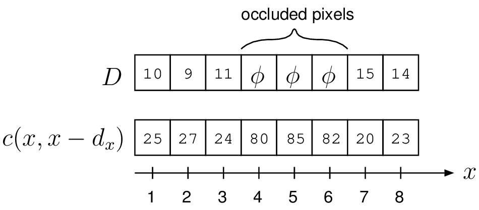
Figure 3.5 Example of the cost calculation defined by Equation (3.9).

Disparity space image.

To estimate the vector of disparity \(D\) and minimize the energy function defined by Equation (3.9), dynamic programming can be employed. The implementation is based on constructing a correlation table, called the Disparity Space Image (DSI) [52]. The DSI structure is a 2D table, of \(d_{max}\) rows and \(w\) columns that contains the matching cost of all pixels (along a scanline) at all possible disparity values. Additionally, the smoothness term is integrated into the DSI as a transition cost between each node of the DSI. Considering the DSI structure as a graph, matching costs and transition costs correspond to node and edges, respectively.

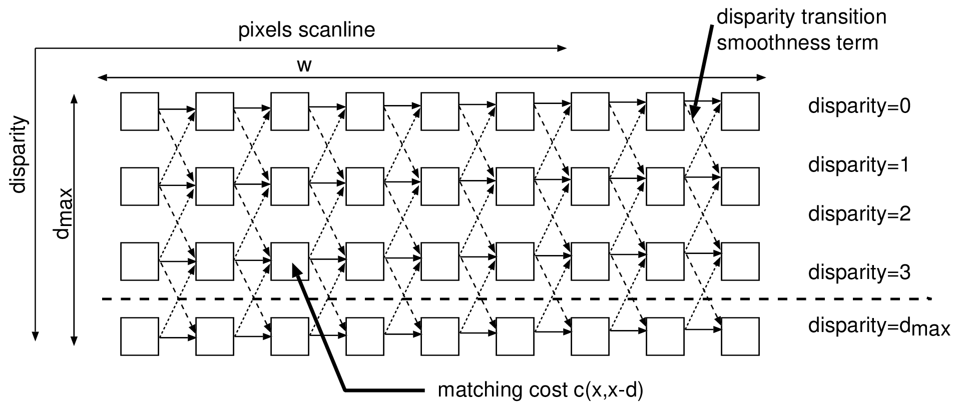
Figure 3.6 DSI structure with all matching costs for all disparity values. Here, a unity disparity change between two consecutive pixels is admissible.

Using dynamic programming, the calculation of the optimal disparity sequence that minimizes Equation (3.9) can be then performed as follows. First, all entries of the DSI structure are initialized using the matching function, i.e., \(DSI(x,d)=c(x,x-d_x)\). Second, a 2D table of cumulated costs \(T(x,d)\) is generated, using the following relation \[T(x,d)=DSI(x,d)+\min_{x_p\in S_{xa}, d_p \in S_{da} } T(x+x_{p},d+d_{p}), (3.14)\] where \(S_{xa}\) and \(S_{da}\) define the “admissible” or “legal” disparity variations between two consecutive pixels, with \(S_{xa}\) and \(S_{da}\) are both a set of integer numbers. In a graph, this corresponds to admissible transitions between nodes. For example, Figure 3.6 illustrates a DSI with the admissible transitions \(S_{xa}=\{-1\}\) and \(S_{da}=\{-1,0,1\}\). Using the array of cumulated costs, the minimum cost sequence can be finally traced back. The algorithm that finds the optimal sequence \(D\) is summarized in Algorithm 1.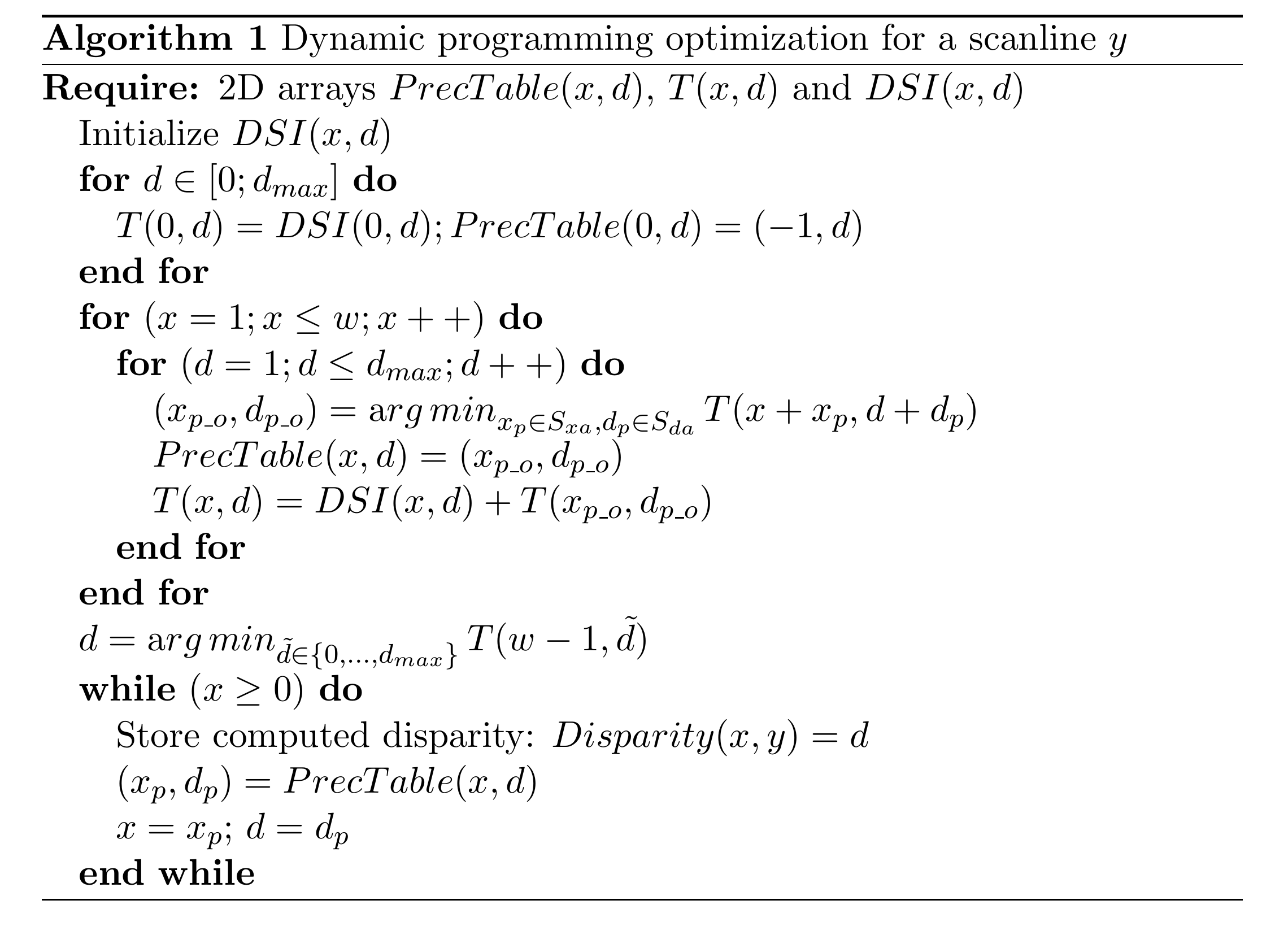

Constraint path.

We now define an admissible path in the DSI that can handle (a) fast disparity variations and (b) occluded pixels. To constrain the admissible edge in the DSI, a solution is to employ an ordering constraint. Such an ordering constraint states that if an object \(\mathcal{A}\) appears at the left of an object \(\mathcal{B}\) in a left image, \(\mathcal{A}\) also appears at the left of \(\mathcal{B}\) in the right image (as defined by Bobick et al. [52]). From this observation, it can be inferred that left-occluded pixels correspond to a disparity increase in the graph while right-occluded pixels correspond to a disparity decrease (see Figure 3.7(a)). Additionally, it should be noted that the DSI edges should allow unmatched pixels to handle occluded pixels. For example, let us consider Figure 3.7(b) that depicts the DSI table at the top, and the corresponding left and right image scanlines and disparity sequence \(D\) at the bottom.

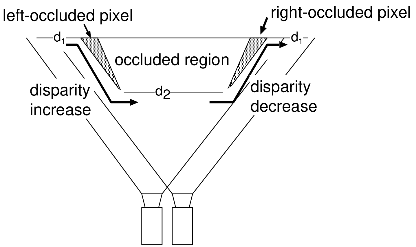
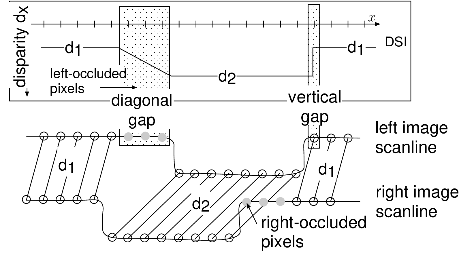
Figure 3.7 (a) Scanning the image from left to right, left- and right-occluded pixels correspond to an increase and decrease of disparity, respectively. (b) Simple DSI (top) with the corresponding scanline profile (bottom) of a left and right image. The admissible disparity transitions correspond to a diagonal gap for left-occluded pixels and a vertical gap for right-occluded pixels.

In Figure 3.7(b), the sequence \(D\) consists of the disparity \(d_1\) and \(d_2\), corresponding to the disparity of the background and foreground objects, respectively. To handle left-occluded pixels, it can be seen that the disparity transition between \(d_1\) and \(d_2\), should allow unmatched pixels. Therefore, left-occluded pixels, giving a decrease of disparity, can be handled by skipping pixels in the left image scanline. This is in accordance with the diagonal gap in the DSI. At the opposite, right-occluded pixels, i.e., decrease of disparity, can be handled by skipping right-occluded pixels, corresponding to a vertical gap in the DSI. Using such admissible edges in the DSI, the algorithm can handle large occluded regions by allowing occluded pixels to remain unmatched. Therefore, the appropriate admissible edges correspond to the path illustrated by Figure [3.8]. Transition costs are indicated as defined by Equation (3.11).

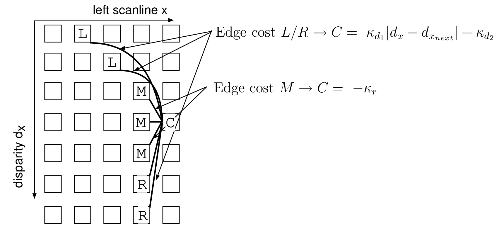Figure 3.8 Admissible edges in the DSI that model left- and right-occluded pixels. Transitions \(L \rightarrow C\) correspond to a diagonal gap to handle left-occluded pixels. Transitions \(R \rightarrow C\) correspond to a vertical gap to handle right-occluded pixels. Transitions \(M \rightarrow C\) correspond to small disparity variations for matching visible pixels.

Experimental results

This section presents experimental results evaluating the accuracy of the reviewed disparity-estimation algorithms. It should be noted that the dis-parity-optimization strategy has a significant impact on the quality of the disparity images. Therefore, we have experimented with several different optimization strategies. More specifically, the presented experiments are performed using three different optimization strategies, with the following characteristics:

1. an optimization strategy based on a WTA algorithm and,

2. a WTA algorithm extended by a cross-checking procedure (see Equation (3.7)), and

3. an optimization strategy based on dynamic programming as described in Section 3.3.3.

All optimization strategies use a fixed matching function (Sum of Absolute Differences) and a fixed support of the matching function (\(5 \times 5\) centered squared window). Each presented disparity image is estimated using fixed parameters. The functions \(B_1(x)\), \(B_2(x)\) define a discontinuity bonus \(B_1(x)=B_2(x)=-75\) if two consecutive pixels show the intensity variations \(|(I(x,y)-I(x+1,y))|>10\). We employed the following set of multi-view images “Teddy”, “Cones”, “Breakdancers”, “Ballet” and “Livingroom” (see Appendix A.2 for a description of the multi-view images data set). For the multi-view images “Breakdancers”, “Ballet” and “Livingroom”, the two employed views were first rectified using the method described in Section 2.4.2. Let us now discuss the resulting estimated disparity images for the three different optimization strategies.

WTA.

First, it can be observed that the “Winner-Take-All” strategy provides an accurate disparity estimation in textured regions. For example, the disparity is correctly estimated in the center region of Figure 3.9(b) and Figure 3.9(f). However, the disadvantages of the WTA strategy are as follows. Looking at the top-right part of Figure 3.9(f), it can observed that the disparity in texture-less regions cannot be accurately estimated. For the sequences “Ballet”,“Breakdancers” and “Livingroom” showing large texture-less regions, the estimated disparity images can be considered as highly inaccurate. These inaccurate depth images are therefore not included in this thesis, as this algorithmic proposal does not give any satisfactory results. A second disadvantage is that the disparity cannot be estimated accurately along object borders where occluded pixels are typically located. For example, the disparity along the left edges of the cones in Figure 3.9(b) cannot be estimated.

WTA extended by cross-checking.

To avoid unreliable disparity estimates, WTA was extented with cross-checking. Considering Figure 3.9(c) and Figure 3.9(g), it can be seen that the cross-checking procedure detects unreliable disparity estimates (shown as blue/black). However, one disadvantage of the procedure is that a too large number of estimates are classified as unreliable. Similar to the WTA experiment without cross-checking, the disparity of the multi-view images “Breakdancers”, “Ballet” and “Livingroom” cannot be estimated and are therefore also not included in this thesis. In the next section, we propose an algorithm that estimates more accurate depth images of which the corresponding calculated depth images will be presented.

One-dimensional optimization.

The one-dimensional dynamic programming optimization provides more reliable disparity estimates with respect to WTA. For example, when observing Figure 3.9(d) and Figure 3.9(h), it can be seen that disparity images correspond to the expected surface of objects in the scene. Furthermore, occluded pixels along the object borders are also detected and correctly handled (see for example the left side of the teddy bear). Additionally, the disparity for the multi-view images “Ballet”,“Breakdancers” and “Livingroom” can be more accurately estimated. For example, observing the disparity of Figure 3.10, it can be seen that the disparities of the checkerboard, the lamp and the tree were correctly estimated. Similar observations can be made by analyzing Figure 3.11 and Figure 3.12. However, all disparity images suffer from scanline streaking artifacts. Such artifacts result from the independent optimization of disparities for each scanline.

(a) Original “Cones” image (b)“WTA”

(c) “WTA” with cross-checking (d)“Dynamic programming”

(e) Original “Teddy” image (f) “WTA”

(g) “WTA” with cross-checking (h) Dynamic programming

Figure 3.9 Estimated disparity images using the “Teddy” and “Cones” multi-view images.

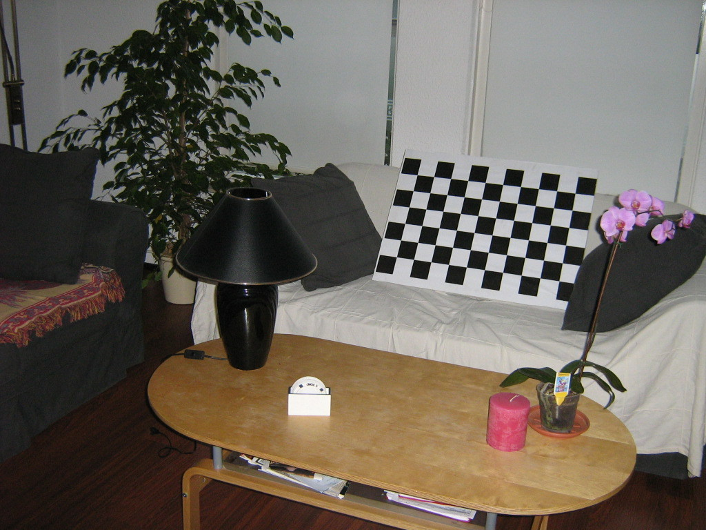
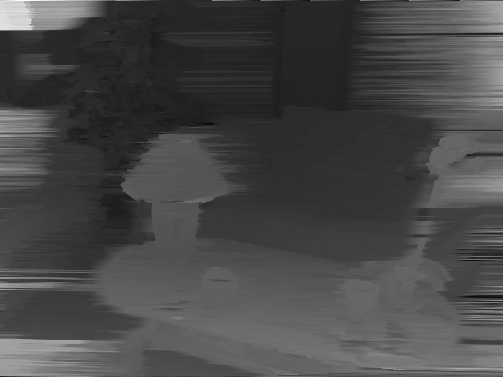
Figure 3.10 (a) View 3 of the “Livingroom” multi-view images data set. (b) Estimated disparity image using the dynamic programming algorithm.

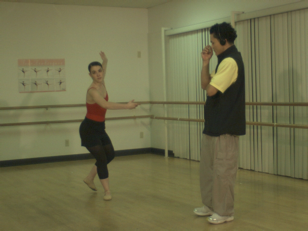
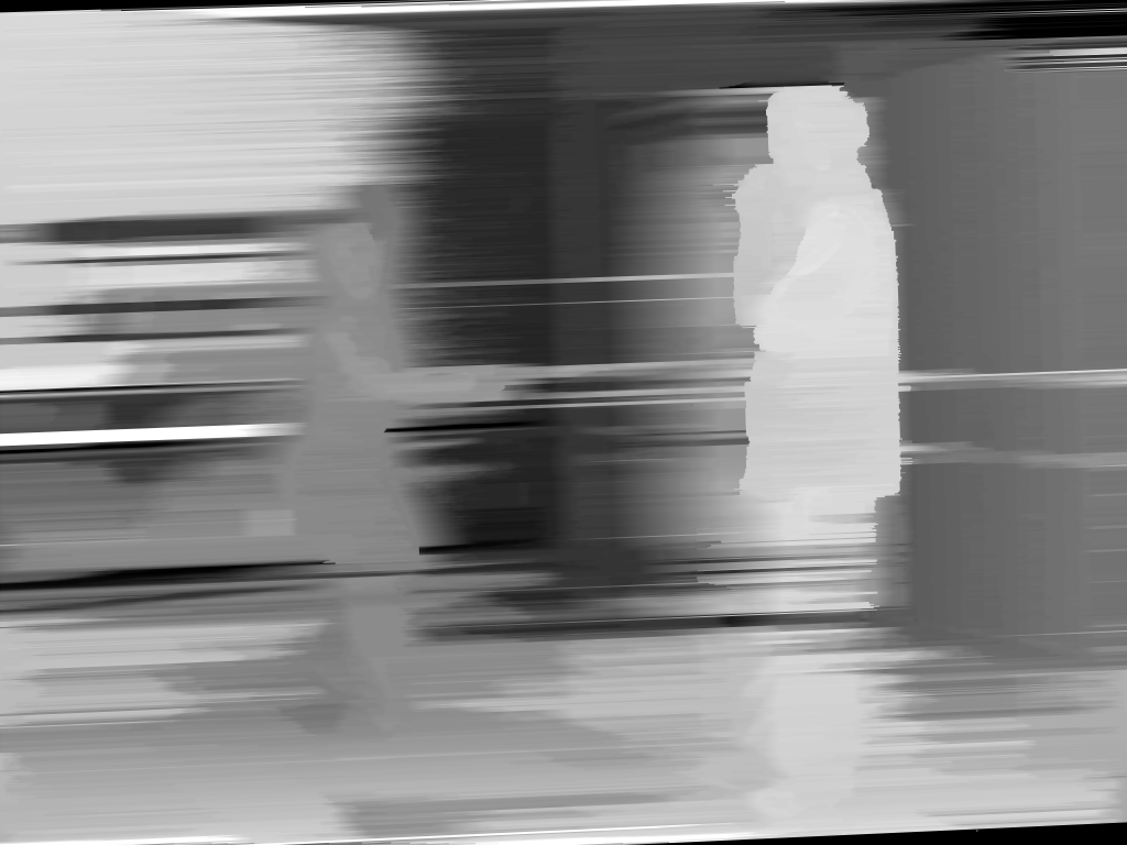
Figure 3.11 (a) View 3 of the “Ballet” multi-view images data set. (b) Estimated disparity image using the dynamic programming algorithm.

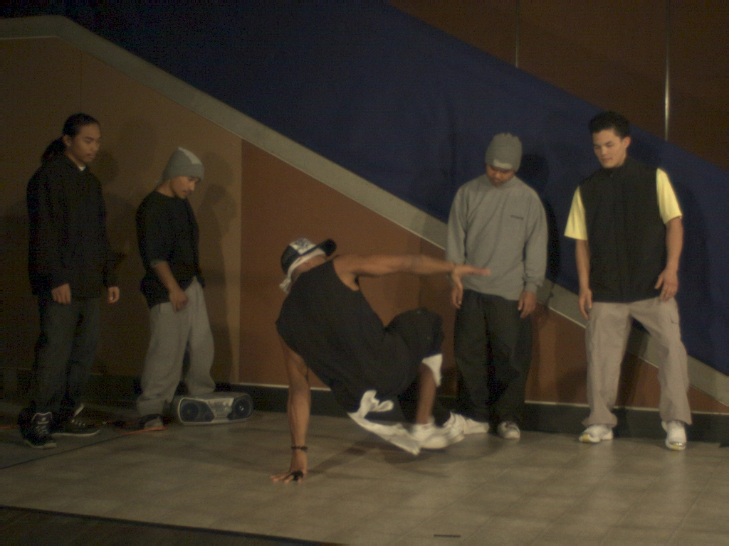
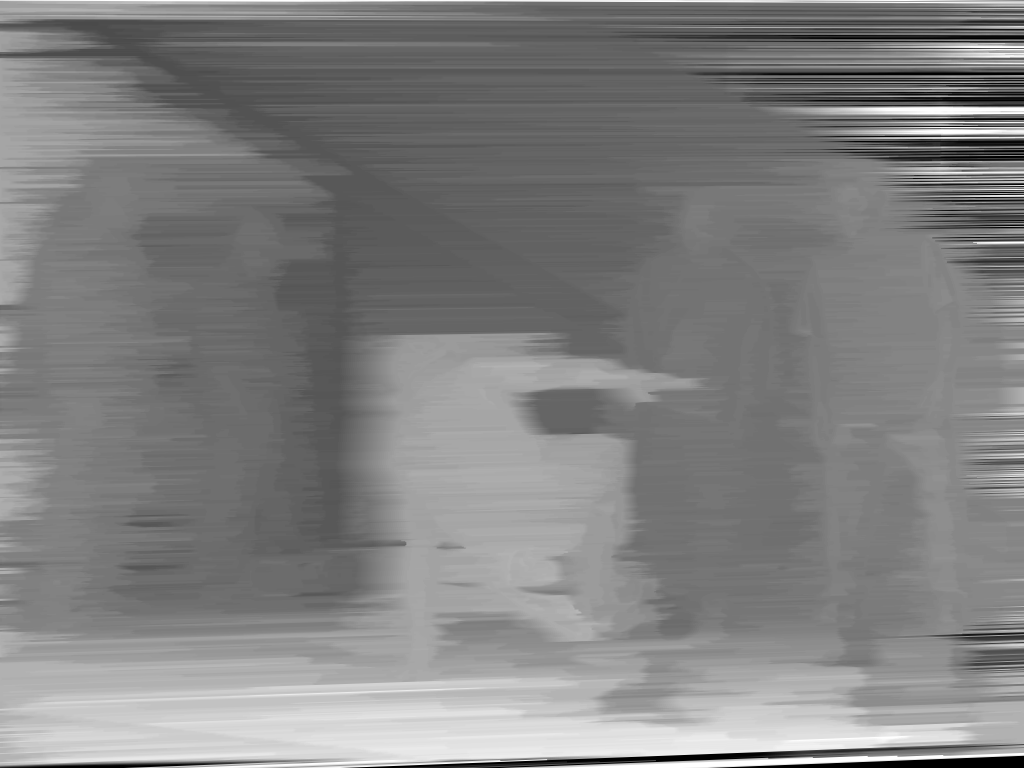
Figure 3.12 (a) View 3 of the “Breakdancers” multi-view images data set. (b) Estimated disparity image using the dynamic programming algorithm.

Intermediate conclusions

The previous experiments lead to a few intermediate conclusions. First, it can noted that the quality of disparity images significantly depends on the characteristics of the input multi-view images. For example, the “Teddy” and “Cones” multi-view images show large colorful and textured regions. As a result, accurate disparity images can be estimated. In contrast with this, the colorless and texture-less characteristics of the “Breakdancers” and “Ballet” multi-view images do not allow an accurate estimation of disparity. To obtain more accurate disparity images for this type of sequences, a one-dimensional optimization strategy was presented. However, while this strategy estimates more accurate disparity values in some regions, significant streaking artifacts are introduced at some other locations. In order to increase the accuracy of the estimation, we explore an increasingly popular approach, employing multiple views of the scene. This approach will addressed in the next section.

Multiple-view depth estimation

Depth estimation for multi-view video coding

The previous section has presented a method that estimates disparity images using two rectified views. Similar approaches [54], [55] were recently investigated to create depth maps for 3D-TV systems. However, in those applications, a pair of images was used to compute the disparity image. In multi-view video, multiple images are available so that an efficient depth estimation algorithm should employ all views available. More specifically, the disadvantages of a pairwise depth estimation algorithm are threefold. First, while multiple views of the scene are available, only two rectified views are employed simultaneously, which degrades performance. Second, because depth images are estimated pairwise, consistency of depth estimates across the views is not enforced. Third, multiple pre-processing (image rectification) and post-processing (disparity-to-depth conversion and image de-rectification) procedures are necessary.

In order to circumvent these three disadvantages, we propose an approach that employs multiple views and estimates the depth using a correlation table similar to the Disparity Space Image (DSI). As in the previous section, the depth is calculated along each scanline using the dynamic programming algorithm from the previous section. Two novel constraints are introduced which are enforcing smooth variations of depth across scanlines and across the views, thereby positively addressing the aforementioned disadvantages. Additionally, no unnecessary conversion from disparity pixels to depth values is required.

Let us now explain the multi-view depth-estimation algorithm that was introduced previously. The presented algorithm calculates a depth image corresponding to a selected reference view \(k_r\) in two steps. In a first step, the 3D world coordinate \((X,Y,Z_c)^T\) of a pixel \(\boldsymbol{p_{k_r}}=(x_{k_r},y_{k_r},1)^T\) (from the reference view) is calculated using a candidate depth value, e.g., \(Z_c\). The 3D world coordinate can be calculated using the back-projection relation (see Equation (2.20)) and be written as \[\left( \begin{array}{c} X\\ Y\\ Z_c \end{array} \right) = \boldsymbol{C_{k_r}}+\lambda_{k_r} \boldsymbol{R_{k_r}}^{-1}\boldsymbol{K_{k_r}}^{-1}\boldsymbol{p_{k_r}}, (3.15)\] where \(\boldsymbol{C_{k_r}}\), \(\boldsymbol{R_{k_r}}\), \(\boldsymbol{K_{k_r}}\) correspond to the parameters of the selected reference camera \(k_r\). It should be emphasized that the 3D point \((X,Y,Z_c)^T\) is described in the world coordinate system that is shared by all cameras. In a second step, the 3D point is projected onto each neighboring view \(k\), providing a corresponding pixel \((x_k,y_k,1)^T\) for each view for which: \[\lambda_k \left( \begin{array}{c} x_k\\ y_k\\ 1 \end{array} \right) = \boldsymbol{P_k} \left( \begin{array}{c} X\\ Y\\ Z_c \end{array} \right), (3.16)\] where \(\boldsymbol{P_k}\) represents the camera parameters of the neighboring camera \(k\). These two steps are repeated for several depth candidates \(Z_c\), so that a corresponding similarity can be measured and stored in a correlation table \(T(x,y,Z_c)\). The algorithm is illustrated by Figure 3.13. It can be noted that this correlation table is similar to the DSI data structure. In practice, an entry in the correlation table \(T(x,y,Z_c)\) is calculated using the sum of the correlation measures over all image views \(I\), specified by \[T(x,y,Z_c)= \sum_{k:k\neq k_r} \sum_{(i,j)\in W} | I_{k_r}(x-i,y-j)-I_k(x_k-i,y_k-j)|. (3.17)\]

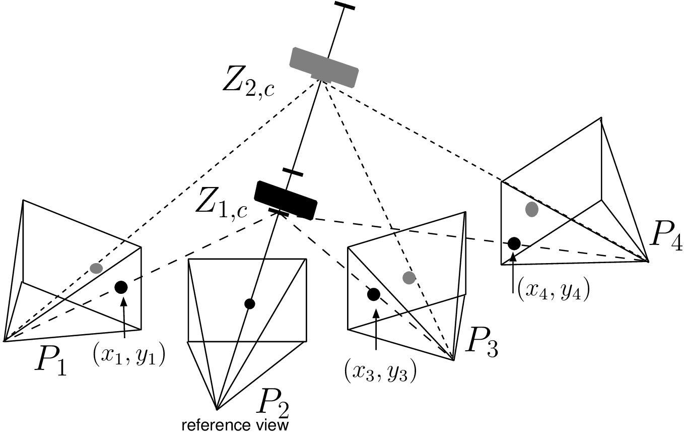
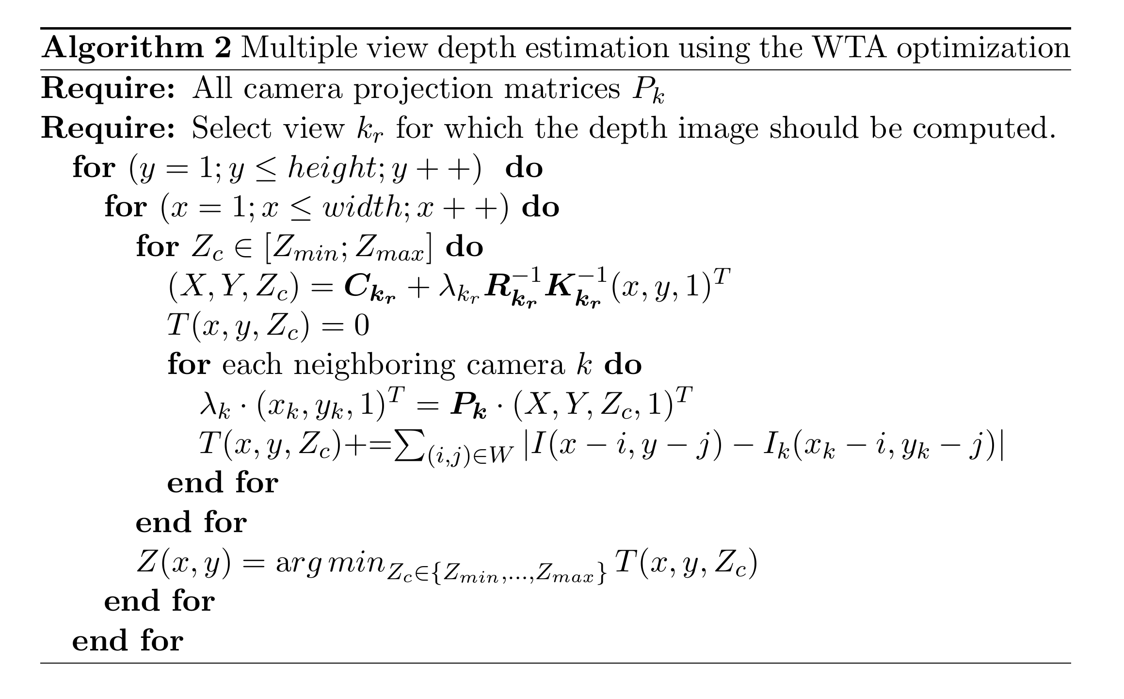
Figure 3.13 Given a reference pixel (black dot), the algorithm tests multiple depth candidates. In this example, the depth candidate \(Z_{2,c}\) yields a grey color in the neighboring views and is therefore not consistent with the black color of the reference pixel. The candidate \(Z_{1,c}\) yields a consistent black color and for this reason, it should be selected as the final depth value.

Using a WTA optimization strategy, the depth value that yields the most consistent (or similar) color across the views is selected as the final estimated depth value. The pseudocode of the algorithm using a WTA optimization is summarized in Algorithm 2.

In the previous section, we have seen that the WTA optimization yields inaccurate depth estimates and noisy depth images. Therefore, we have experimented earlier with a dynamic programming optimization strategy to enforce smooth variations of the depth, which has led to streaking artifacts. In the next section, we impose two additional constraints to obtain more accurate depth estimates.

Two-pass optimization strategy

To enforce smooth depth variations within the image and between the images, we present two novel constraints: (1) smooth variations of depth values across image scanlines and (2) consistent depth values across the views. To combine these constraints with the dynamic programming algorithm, we employ two penalty costs, namely an inter-line penalty cost and an inter-view penalty cost that both extend the cost function \(E(D)\) previously defined by Equation (3.11). The proposed algorithm estimates a depth image by minimizing two different objective cost functions in two passes. In a first pass, a depth image is estimated for each view with the constraint that consecutive image scanlines should show smooth depth variations across the lines. The purpose of this pass is to generate one initialization depth image for each view without streaking artifacts. We denote the objective function for one view at the first pass as \[E_{pass\ 1}(D)=E(D)+ E_{smooth\ 1}(D), (3.18)\] where \(E_{smooth\ 1}(D)\) is defined in the following paragraph. This computation is repeated for each view. In a second pass, a depth image is re-estimated for each view with the constraint that an object should have consistent world depth values in all depth images estimated during the first pass. The aim of this second pass is to refine the initialization depth images from the first pass such that the final depth images are consistent across the views. We denote the objective function at the second pass as \[E_{pass\ 2}(D)=E(D)+ E_{smooth\ 2}(D), (3.19)\] where \(E_{smooth\ 2}(D)\) is also defined in the sequel.

Pass 1. Consistent depth values across scanlines.

To enforce smooth variations of depth values across scanlines, we introduce an inter-line penalty cost. Practically, the objective cost function integrating the inter-line penalty cost can be written as \[E_{smooth\ 1}(D)= \sum_{x} \underbrace{\kappa_l \cdot |Z_{k_r}(x,y)-Z_{k_r}(x,y-1)|}_{\textrm{inter-line penalty cost}}, (3.20)\] where \(D\) is the vector of depth values \(Z_{k_r}(x,y)\) along a scanline, \(Z_{k_r}(x,y)\) the estimated depth at position \((x,y)\) in the reference image with index \(k_r\) and \(\kappa_l\) the inter-line penalty parameter (typically a scalar). The index of the reference view \(k_r\) varies between \(1\leq k_r \leq N\), for an \(N\)-view data set.

Pass 2. Consistent depth values across the views.

In a second pass, the depth is refined for each view by incorporating a cost that penalizes inconsistent depth values across the views into the objective cost function \( E_{smooth\ 2}(D)\) (see Figure (3.14)). Similar to the first constraint, the objective function that integrates the inter-line and inter-view penalty costs is written as \[\begin{aligned} E_{smooth\ 2}(D)& =& \sum_{x}\bigg( \kappa_l \cdot |Z_{k_r}(x,y)-Z_{k_r}(x,y-1)| + \\ & &\underbrace{\sum_{k,k\neq k_r} \kappa_v \cdot |Z_{k_r}(x,y)-Z_k(x_k,y_k)|}_{\textrm{inter-view penalty cost}} \bigg), (3.22)\end{aligned}\] where \(\kappa_v\) corresponds to the inter-view penalty parameter. The depth \(Z_{k_r}(x, y)\) and \(Z_{k}(x_k ,y_k)\) correspond to the depth in the reference view with index \(k_r\) and neighboring views \(k\), respectively. It should be noted that both depth values \(Z_{k_r}(x, y)\) and \(Z_k(x_k, y_k)\) are described in the world coordinate system, thereby enabling a direct comparison. Finally, to determine the value of the depth \(Z_{k}(x_k, y_k)\) in the neighboring views, the pixel \((x,y)\) is projected onto the neighboring image planes \(k\), which provides the pixel position \((x_k, y_k)\) and the corresponding depth \(Z_{k}(x_k, y_k)\) that was calculated during the first pass.

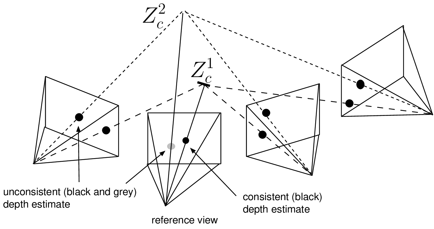
Figure 3.14 In this example, a correct depth value (black dot in the reference view) is consistent across the views. Alternatively, an incorrect depth value (grey dot in the reference view) leads to inconsistent depth values across the views.

Admissible path in the DSI.

To optimize the previous objective functions \(E_{pass\ 1}(D)\) and \(E_{pass\ 2}(D)\), the dynamic programming algorithm is employed. In Section [sec:dyn_prog], we have seen that the optimal path in the DSI is derived from the ordering constraint. However, the ordering constraint cannot be employed in the extended case of multiple-view depth estimation because no left or right camera position is assumed. We therefore employ an admissible edge that enables an arbitrary increase or decrease of depth values. The admissible edges in the DSI are portrayed by Figure 3.15.

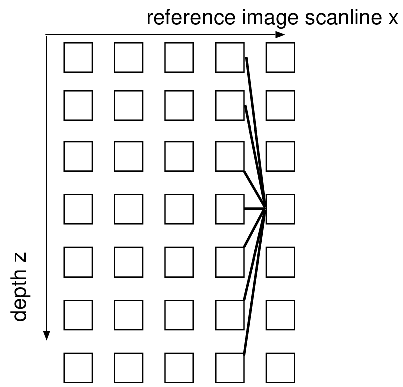
Figure 3.15 Because the ordering constraint cannot be employed in the extended case of depth estimation with multiple views, the admissible edges illustrated above are used, allowing all possible transitions.

Depth sampling of the 3D space

For 3D sampling, it should be noted that there exists a dependency between the depth of an object and its corresponding resolution in the image. For example, far and near objects are seen as small and large in the image, respectively. A near object can therefore be observed with higher resolution than a far object so that the depth resolution of a near object should be higher than that of a far object. In this context, we employ the plenoptic sampling framework [56]. The idea of the plenoptic sampling framework is to employ a non-linear quantization of the depth between a minimum and maximum depth \(Z_{min}\) and \(Z_{max}\) (see Figure 3.16).

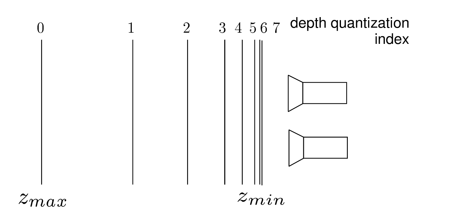
Figure 3.16 Non-linear depth sampling of the 3D space.

More specifically, the depth \(Z_i\) for a quantization index \(i\) can be written as \[\frac{1}{Z_i} = \eta_i \frac{1}{Z_{min}}+(1-\eta_i)\frac{1}{Z_{max}}, (3.23)\] with \[\eta_i=\frac{i-0.5}{N_d}\textrm{ and } i=1,...,N_d, (3.24)\] where \(N_d\) corresponds to the maximum number of depth values/layers. Alternatively, the quantization index \(i\) of a depth value \(Z_i\) can be written as \[i=\lfloor N_d \frac{ Z_i^{-1}-Z_{max}^{-1} }{ Z_{min}^{-1} -Z_{max}^{-1} } +0.5 \rfloor. (3.25)\] The depth of a pixel can be therefore efficiently stored and represented using the corresponding quantization index \(i\). In the case that \(256\) possible depth values are employed, the depth quantization index can be represented using an \(8\)-bit pixel format and stored using a standard \(8\) bits per pixel image.

Depth image post-processing

Having calculated a depth image for each view, an optional task is to apply a noise-reduction algorithm as a last post-processing step. Typically, this noise-reduction stage noticeably improves the quality of depth images at a limited computational cost. For example, based on the assumption that depth pixels vary smoothly at the object surfaces, a simple noise-reduction algorithm consists of filtering noisy pixels that have low spatial correlation with neighboring pixels. However, the assumption of smoothly varying depth pixels is invalid at object borders (edges). Therefore, the challenge is to filter noisy pixels (outliers) while preserving the accuracy of depth pixels along object borders. To implement this concept, we propose in this section a depth-image denoising algorithm that actively supports smooth regions in the depth image while preserving sharp depth discontinuities along the object borders.

The proposed noise-reduction algorithm proceeds in two stages. At the first stage, a color segmentation is applied to the texture image that corresponds to the considered depth image. The intuitive idea underlying this first stage is that the resulting segments, which delineate the object contours, correspond to a piece/portion of the object surfaces. Because object surfaces show smooth regions in the depth image, the corresponding depth image segments can be approximated by a piecewise-linear function [45]. Figure 3.17 shows an example of a color-segmented image obtained using the watershed segmentation algorithm [57].

figure 3.18 (a) Original texture image and (b) corresponding segmented image using a watershed segmentation algorithm. Note that the depth of each segment, e.g., the background wall, can be modeled by a piecewise-linear function.

At the second stage, a piecewise-linear function which models the object surfaces is estimated for each image segment. To calculate the linear function parameters of each segment, we apply a robust estimation method, i.e., the RANdom SAmple Consensus (RANSAC) algorithm [58]. The advantage of this algorithm is that it can estimate parameters even if the data is disturbed by a large number of outliers, i.e., noisy depth pixels. Because we assume that the data fits to a piecewise-linear function, three pixels are sufficient to calculate a plane and thus the corresponding parameters. The RANSAC algorithm first randomly selects three pixels, which are used to compute candidate parameters of the linear (planar) function. The algorithm then counts the number of pixels that fit to this model (inliers). This procedure is repeated several times and finally, the parameters with the largest support are selected as the parameters for the considered image segment (see a one-dimensional example in Figure 3.18). The robust RANSAC estimation of piecewise-linear function parameters is then performed for all image segments. The advantages of the depth image post-processing step are twofold. First, because the depth is accurately estimated especially at object borders, a high-quality image can be rendered (this property of image rendering will be discussed in Chapter 4). Second, the resulting depth image presents smoothly varying properties and thus can be encoded efficiently. Note that this property will be exploited in Chapter 6 for the coding of depth images.

Figure 3.18 Two samples are randomly selected to compute a candidate model indicated by the solid line. Input data close to the line candidate is considered as inliers (black dots between dotted lines). Fig. 3.18(a) and Fig. 3.18(b) show two candidate models with a small and a high number of inliers, respectively. The model with the largest number of inliers is selected.

Experimental results

In this section, we present experimental results evaluating the accuracy of the depth estimation algorithm from the previous section. We especially focus on the challenging problem of estimating depth images using texture-less and colorless multi-view images. For this reason, we employ the multi-view images “Breakdancers”, “Ballet” and “Livingroom”, featuring these properties. Note that because the calibration parameters are necessary for multi-view depth estimation, the depth images “Teddy” and “Cones” are not estimated (no parameters available). For each presented depth image, the parameters are empirically determined and not specifically adapted to each data set. We first provide an objective evaluation and, second, proceed by subjectively assessing the depth image quality. Finally, we compare the quality of the calculated depth images with two alternative methods, based on a two-dimensional optimization strategy.

A. Objective evaluation

For the objective evaluation of the depth image quality, we employ an image rendering method that synthesizes virtual views using the calculated depth image. This technique is based on the notion that the quality of the rendered image depends on the accuracy of the estimated depth image. Specifically, the more accurate a depth image is, the higher the rendering quality becomes. In our experiments, the synthesis of virtual images is carried out using the relief texture rendering algorithm, which will be presented in Chapter 4. In the presented experiments, we use a post-processing step as defined in Section 3.4.4. To evaluate the quality of rendered images, a synthetic image is rendered at the same position and orientation of a selected reference camera ⁹. By comparing the synthetic image \(I_s\) with the reference image \(I_r\), the Peak Signal-Noise Ratio (\(\mathit{PSNR_{rs}}\)) can be calculated by \[\mathit{PSNR_{rs}} = 10 \cdot \log_{10} \left( \frac{255^2}{\mathit{MSE_{rs}}} \right), (3.26)\] where the Mean Squared Error (MSE) is computed by the following equation: \[\mathit{MSE_{rs}} = \frac{1}{w \cdot h}\sum_{i=1}^{w}\sum_{j=1}^{h} ||I_r(i,j) - I_s(i,j)||^2, (3.27)\] with \(w\) and \(h\) corresponding to the width and the height of the images, respectively. Note that the \(\mathit{PSNR_{rs}}\) metric has shown some limitations for evaluating the image quality because it does not match the human subjective perception. However, this is the only simple alternative image quality metric that has been widely accepted and used by the research community (also adopted in key literature [59] on rendering). Besides computing this metric, we will also comment on the subjective depth image quality. The differences between the objective (\(\mathit{PSNR_{rs}}\)) and subjective rendering quality will be illustrated by Figure 6.11 in Chapter 6. The discussed results are compared in a relative sense to the conventional algorithm addressed earlier in this chapter. Up till now, results on multi-view depth estimation in literature are still being presented in a subjective discussion. To avoid the ambiguity of such a discussion, we have presented here a well-defined measurement for estimating the quality of depth images. This indirect method, based on rendering quality evaluation, gives a less precise evaluation of the depth quality than a direct method based on a comparison with, e.g., a ground-truth depth image. However, calibrated ground-truth multi-view depth images are presently not available to the research community. Additionally, it may be argued that the image rendering quality is more important than the quality of the depth images because depth images are not visualized by the user (as opposed to the rendered images).

Let us now discuss the rendering-quality measurements summarized in Table 3.1. First, it can be seen that the proposed algorithm that uses multiple views to estimate depth images consistently and significantly outperforms the two-view depth-estimation algorithm. For example, an image-quality improvement of 2.9 dB, 3.2 dB and 0.3 dB can be observed for the “Breakdancers”, “Ballet” and “Livingroom” sequences, respectively. The lower improvement for the “Livingroom” sequence is mainly due to an inaccurate texture rendering of the scene, and especially, an inaccurate rendering of the background tree. Considering the applications of 3D-TV and free-viewpoint video, the contributed two-pass algorithm clearly enables high-quality rendering, thereby facilitating the reconstruction of a high-quality depth signal.

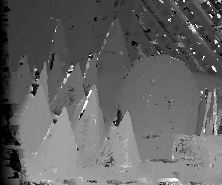
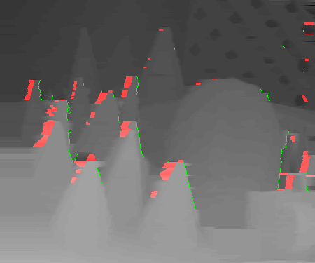
B. Subjective evaluation

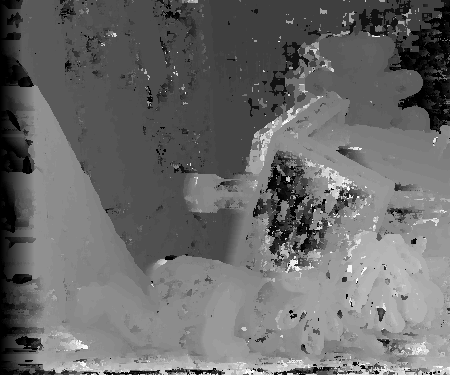
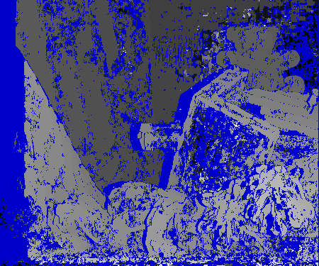
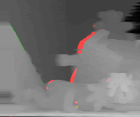
Figures 3.19, 3.20 and 3.21 enable a discussion on the subjective quality of the estimated depth images using the proposed two-pass algorithm. We assess the quality of the depth images prior to the post-processing step. First, it can be observed that, prior to the post-processing step, the two-pass algorithm leads to more consistent depth values across the lines, so the annoying streaking artifacts are reduced leading to a significant perceptual improvement. For example, observing Figure 3.19(a), it can be noted that the two-pass algorithm leaves over little streaking artifacts in the image. Similar conclusions can be drawn by observing Figure 3.20(b) and Figure 3.21(b), albeit there is still fuzzyness around the objects. Second, it can be noted that the depth of colorless and texture-less regions can be accurately estimated. For example, the depth values of the texture-less walls in Figure 3.19(b) and Figure 3.21(b) are correctly estimated and do not suffer from streaking artifacts. Additionally, the depth of very thin objects such as the flower stalk, can be correctly estimated (see Figure 3.19(b)). Such an accurate result is obtained by using multiple views simultaneously and by enforcing consistent depth values across the views. However, several estimation errors occur at object boundaries which correspond to depth discontinuities (e.g., borders of the dancer in Figure 3.20(b)). Let us now assess the quality of the depth images after the post-processing step. As expected, it can be seen in Figures 3.19(c), 3.20(c) and 3.21(c) that the post-processed depth images depict piecewise-linear regions delineated by sharp boundaries. For example, Figure 3.19(c) shows that the depth along the border of the table is accurately delineated. Similar conclusions can be drawn by comparing Figure 3.20(b) with Figure 3.20(c) and Figure 3.21(b) with Figure 3.21(c). Thus, the introduced post-processing step clearly removes noisy pixels while preserving the edges along objects in the depth image.

C. Subjective comparisons with alternative methods

Next, we have compared the quality of the calculated depth images with two alternative methods based on a two-dimensional optimization strategy (see Section 3.3.3). Note that only a few alternative contributions exist, employing the complex “Breakdancers” and “Ballet” multi-view sequences. We have found only two proposals that employ either both sequences [50], or one sequence only (“Breakdancers”) [51].

The first alternative proposal is based on a modified plane sweeping algorithm [51]. By subjectively comparing Figure 3.20(c) and Figure 3.22(a) it can be seen that the method proposed in this thesis results in a slightly more accurate depth image ¹⁰. For example, the competing method generates some depth artifacts in the occluded region along the arm of the breakdancer. Additionally, the proposed method enables an accurate depth estimation along the delineation between the background wall and the rightmost person (see Figure 3.20(c)). At the opposite, the competing method does not allow the visualization of the discussed depth discontinuity (along the person delineation).

The second alternative proposal [50] performs an over-segmentation of the texture image, and calculates the depth of each segment using a belief propagation algorithm. For the “Breakdancers” sequence, it can be seen that both methods lead to a similar depth image quality. For example, the depth discontinuity between the breakdancer and the background wall is accurately estimated in both cases (see Figure 3.20(c) and Figure 3.22(b)). However, for the “Ballet” sequence, it can be noticed that the proposed method yields a less accurate depth image. For example, the depth discontinuity along the foreground person is better calculated by the alternative proposal (see Figure 3.22(c)).

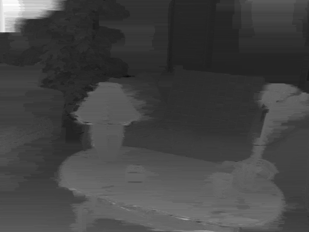
Figure 3.19 (a) View 3 of the “Livingroom” sequence. Estimated depth images (b) prior to post-processing and (c) after the post-processing step.

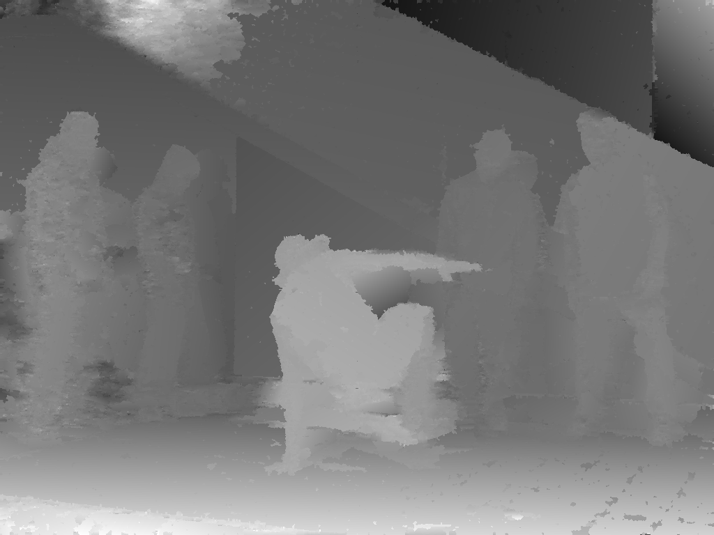
Figure 3.20 (a) View 3 of the “Breakdancers” sequence. Estimated depth images (b) prior to post-processing and (c) after the post-processing step.

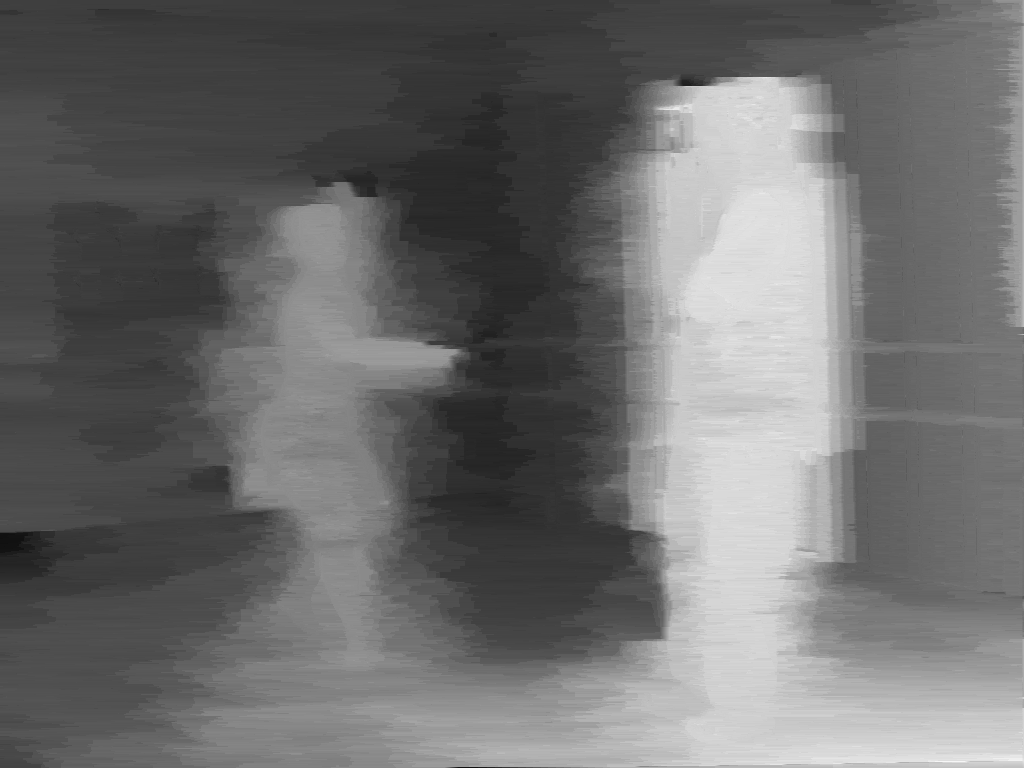
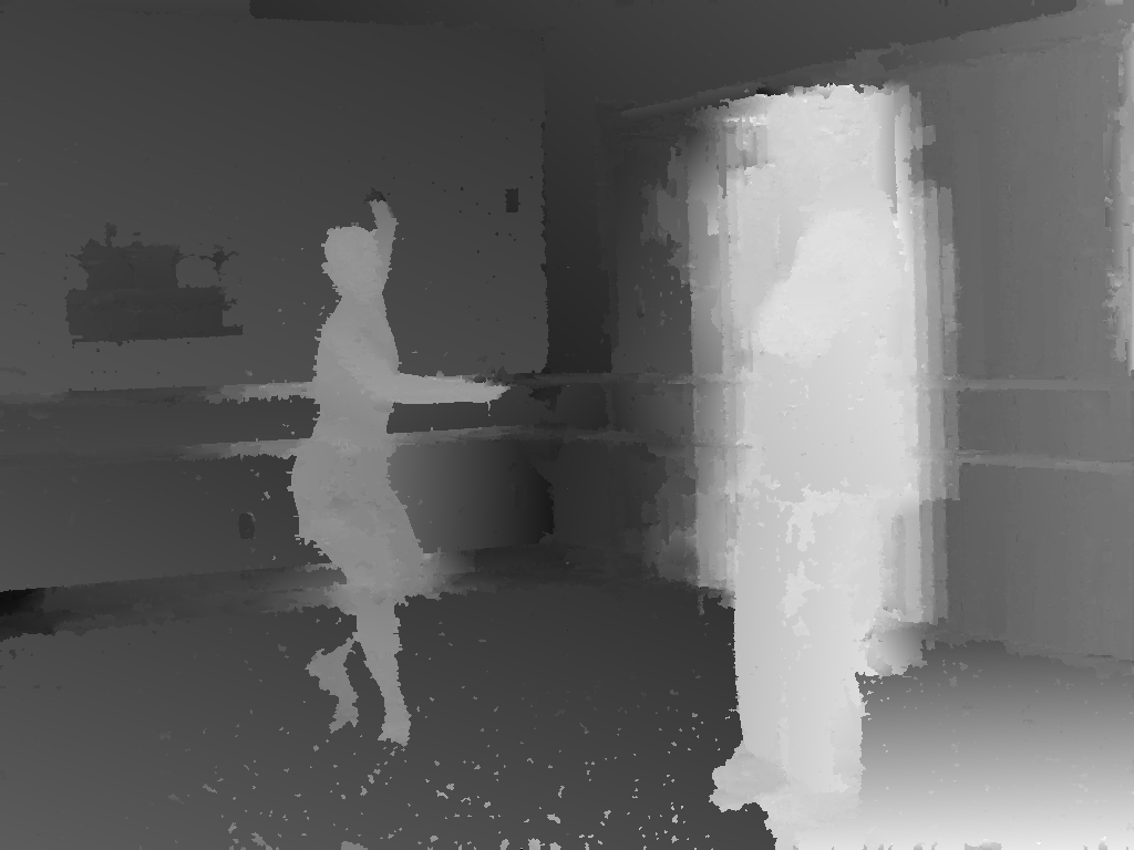
Figure 3.21 (a) View 3 of the “Ballet” sequence. Estimated depth images (b) prior to post-processing and (c) after the post-processing step.

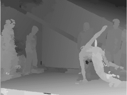
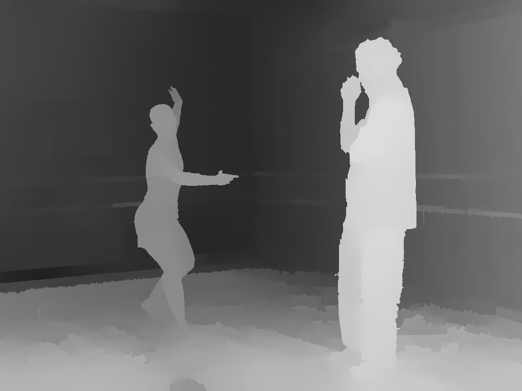
Figure 3.22 Depth images calculated using the algorithm based on (a) plane-sweeping [51] and (b) (c) over-segmentation [8].

Summary and conclusions

Using the geometry of multiple views, we have derived the basic principles employed to calculate the depth using two views and multiple views. We have discussed two popular optimization strategies employed for estimating disparity images: WTA and and a one-dimensional optimization strategy based on dynamic programming. In the presented experiments, we have highlighted three important disadvantages of the two previously mentioned depth-estimation algorithms: (1) only two rectified views are employed simultaneously, (2) consistency of depth estimates across the views is not enforced and (3) multiple pre-processing (image rectification) and post-processing (disparity-to-depth conversion and image de-rectification) procedures are necessary. To address these problems, in the last section, we have introduced an alternative depth image estimation algorithm. The proposed algorithm is based on two novel constraints, i.e., an inter-line and an inter-view smoothness constraint, which enforce smooth variations of depth values across scanlines and consistent depth values across the views. The first pass of the algorithm serves as an estimate for depth image initialization, whereas the second pass refines the initial depth images by enforcing consistent depth across the views. Experiments have shown that especially the second pass provides a noticeable quality improvement by detecting and removing fuzzy outliers that are not consistent across the views. We have shown than both smoothness constraints can be efficiently integrated into the one-dimensional optimization dynamic programming algorithm. Experiments have shown that the proposed constraints yield reasonably accurate depth values for the critical case of texture-less and colorless multi-view images.

At this point, it is relevant to come back on the initial requirements stated in the introduction of this chapter. The primary requirement of the depth estimation algorithm is that it should lead to accurate depth images featuring smooth regions delineated by sharp edges (piecewise linear regions). To fulfill this requirement, we have proposed a post-processing step that segments the texture image into regions of linear depth. The above-discussed piecewise linear property of the depth images is highly relevant for the coding of depth images, as discussed in Chapter [chapter:depth_compression]. The second important contribution and initial requirement is that the resulting depth images should be consistent across the views. The proposed two-pass algorithm explicitly detects and removes inconsistent depth estimates to enforce consistency. It will be seen in Chapter 5, that such an inter-view consistency can be beneficially exploited for compression purposes, where the inter-view consistency corresponds to an inter-view redundancy.

References

[37] D. Scharstein, R. Szeliski, and R. Zabih, “A taxonomy and evaluation of dense two-frame stereo correspondence algorithms,” in IEEE workshop on stereo and multi-baseline vision, 2001, pp. 131–140.
[38] F. Devernay, “Vision stéréoscopique et propriétés différentielles des surfaces,” PhD thesis, Ecole Polytechnique, Palaiseau, France, 1997.
[39] S. Birchfield and C. Tomasi, “A pixel dissimilarity measure that is insensitive to image sampling,” IEEE Transactions on Pattern Analysis and Machine Intelligence, vol. 20, no. 4, pp. 401–406, 1998.
[40] T. Kanade and M. Okutomi, “A stereo matching algorithm with an adaptive window: Theory and experiment,” IEEE Transactions on Pattern Analysis and Machine Intelligence, vol. 16, no. 9, pp. 920–932, 1994.
[41] A. Fusiello, V. Roberto, and E. Trucco, “Efficient stereo with multiple windowing,” in IEEE conference on computer vision and pattern recognition, 1997, pp. 858–863.
[42] S. B. Kang, R. Szeliski, and J. Chai, “Handling occlusions in dense multi-view stereo,” in IEEE conference computer vision and pattern recognition, 2001, vol. 1, pp. I–103–I–110.
[43] H. Tao, H. S. Sawhney, and R. Kumar, “A global matching framework for stereo computation,” in IEEE international conference on computer vision, 2001, vol. 1, pp. 532–539.
[44] M. Bleyer and M. Gelautz, “A layered stereo matching algorithm using image segmentation and global visibility constraints,” ISPRS Journal of Photogrammetry and Remote Sensing, vol. 59, no. 3, pp. 128–150, 2005.
[45] H. Tao and H. S. Sawhney, “Global matching criterion and color segmentation based stereo,” in IEEE workshop on applications of computer vision, 2000, pp. 246–253.
[46] S. Birchfield and C. Tomasi, “Depth discontinuities by pixel-to-pixel stereo,” International Journal of Computer Vision, vol. 35, no. 3, pp. 269–293, 1999.
[47] Y. Boykov, O. Veksler, and R. Zabih, “Fast approximate energy minimization via graph cuts,” IEEE Transactions on Pattern Analysis and Machine Intelligence, vol. 23, no. 11, pp. 1222–1239, 2001.
[48] V. Kolmogorov and R. Zabih, “Computing visual correspondence with occlusions via graph cuts,” in IEEE international conference on computer vision, 2006, vol. 2, pp. 508–515.
[49] J. Sun, N.-N. Zheng, and H.-Y. Shum, “Stereo matching using belief propagation,” IEEE Transactions on Pattern Analysis and Machine Intelligence, vol. 25, no. 7, pp. 787–800, 2003.
[50] C. L. Zitnick and S. B. Kang, “Stereo for image-based rendering using image over-segmentation,” International Journal of Computer Vision, vol. 75, no. 1, pp. 49–65, October 2007.
[51] C. Cigla, X. Zabulis, and A. A. Alatan, “Region-based dense depth extraction from multi-view video,” in IEEE international conference on image processing, 2007, vol. 5, pp. V213–V216.
[52] A. F. Bobick and S. S. Intille, “Large occlusion stereo,” International Journal of Computer Vision, vol. 33, no. 3, pp. 181–200, 1999.
[53] I. J. Cox, S. L. Hingorani, S. B. Rao, and B. M. Maggs, “A maximum likelihood stereo algorithm,” Computer Vision and Image Understanding, vol. 63, no. 3, pp. 542–567, 1996.
[54] P. Kauff et al., “Depth map creation and image-based rendering for advanced 3DTV services providing interoperability and scalability,” Signal Processing: Image Communication, vol. 22, no. 2, pp. 217–234, 2007.
[55] S. Yea and A. Vetro, “CE3: Study on depth issues.” ISO/IEC JTC1/SC29/WG11 and ITU SG16 Q.6 JVT-X073, Geneva, Switzerland, 2007.
[56] J.-X. Chai, S.-C. Chan, H.-Y. Shum, and X. Tong, “Plenoptic sampling,” in International conference on computer graphics and interactive techniques, (acm siggraph), 2000, pp. 307–318.
[57] J. B. Roerdink and A. Meijster, “The watershed transform: Definitions, algorithms and parallelization strategies,” FUNDINF: Fundamenta Informatica, vol. 41, 2000.
[58] M. A. Fischler and R. C. Bolles, “Random sample consensus: A paradigm for model fitting with applications to image analysis and automated cartography,” Communications of the ACM, vol. 24, no. 6, pp. 381–395, 1981.
[59] M. Levoy and P. Hanrahan, “Light field rendering,” in International conference on computer graphics and interactive techniques, (acm siggraph), 1996, pp. 31–42.