Projective Geometry
This chapter starts with an introduction to projective geometry which is of significant importance for the acquisition of 3D images. Using the projective geometry framework, we describe the pinhole camera model that establishes the geometric relationship between a point in the 3D world and its corresponding position in the 2D image. In particular, internal and external camera parameters that indicate the position and settings of the camera are introduced. To estimate these parameters, i.e., calibrate the camera, a practical camera calibration method is then reviewed. We proceed by reviewing the extension of the geometric framework from the single-view to the two-view camera case and finally provide a summary of the parameters and notations employed throughout in this thesis.
Projective geometry
Projective geometry serves as a mathematical framework for 3D multi-view imaging and 3D computer graphics. It is used to model the image-formation process, generate synthetic images, or reconstruct 3D objects from multiple images. To model lines, planes or points in a 3D space, usually the Euclidean geometry is employed. However, a disadvantage of the Euclidean geometry is that points at infinity cannot be modeled and are considered as a special case. This special case can be illustrated by using a perspective drawing of two parallel lines. In perspective, two parallel lines, e.g., a railroad track, meet at infinity at the vanishing point (see Figure 2.1). However, the intersection of the parallel lines at infinity is not easily modeled by the Euclidean geometry. A second disadvantage of Euclidean geometry is that projecting a 3D point onto an image plane requires a perspective scaling operation. As the scale factor is a parameter, the perspective scaling requires a division that becomes a non-linear operation. Therefore, the use of the Euclidean geometry should be avoided.
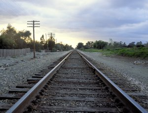
Figure 2.1 Two parallel rails intersect in the image plane at the vanishing point.
Projective geometry constitutes an attractive framework to circumvent the above disadvantages of the Euclidean geometry. In Euclidean space, a point defined in three dimensions is represented by a \(3\)-element vector \((X,Y,Z)^T\). In the projective space, the same point is described using a \(4\)-element vector \((X_1,X_2,X_3,X_4)^T\) such that \[\begin{aligned} X=X_1/X_4,&Y=X_2/X_4, & Z=X_3/X_4,\end{aligned}\] where \(X_4 \neq 0\). Usually, the coordinates \((X,Y,Z)^T\) and \((X_1,X_2,X_3,X_4)^T\) are called inhomogeneous coordinates and homogeneous coordinates, respectively.
As a generalization, the mapping from a point in the \(n\)-dimensional Euclidean space to an \((n+1)\)-dimensional projective space can be written as \[\underbrace{(X_1,X_2,...,X_n)^T}_{Euclidean\ space} \to \underbrace{(\lambda X_1,\lambda X_2,...,\lambda X_n,\lambda)^T}_{projective\ space}, \label{eq:inhomogeneous}\] where \(\lambda \neq 0\) corresponds to a free scaling parameter. This free scaling parameter \(\lambda\) is often called the homogeneous scaling factor. Using the presented projective geometry framework, we now introduce the pinhole camera model.
Pinhole camera model
In this section, we describe the image acquisition process known as the pinhole camera model, which is regularly employed as a basis in this thesis. More specifically, we first discuss the model that integrates the internal or intrinsic camera parameters, such as the focal length and the lens distortion. Secondly, we extendn the presented simple camera model to integrate external or extrinsic camera parameters corresponding to the position and orientation of the camera.
Intrinsic camera parameters
The pinhole camera model defines the geometric relationship between a 3D point and its 2D corresponding projection onto the image plane. When using a pinhole camera model, this geometric mapping from 3D to 2D is called a perspective projection. We denote the center of the perspective projection (the point in which all the rays intersect) as the optical center or camera center and the line perpendicular to the image plane passing through the optical center as the optical axis (see Figure 2.2). Additionally, the intersection point of the image plane with the optical axis is called the principal point. The pinhole camera that models a perspective projection of 3D points onto the image plane can be described as follows.
A. Perspective projection using homogeneous coordinates
Let us consider a camera with the optical axis being collinear to the \(Z_{cam}\)-axis and the optical center being located at the origin of a 3D coordinate system (see Figure 2.2).

Figure 2.2 The ideal pinhole camera model describes the relationship between a 3D point \((X,Y,Z)^T\) and its corresponding 2D projection \((u,v)\) onto the image plane.
The projection of a 3D world point \((X,Y,Z)^T\) onto the image plane at pixel position \((u,v)^T\) can be written as \[u=\frac{Xf}{Z} \textrm { and } v=\frac{Yf}{Z},\] where \(f\) denotes the focal length. To avoid such a non-linear division operation, the previous relation can be reformulated using the projective geometry framework, as \[\begin{aligned} (\lambda u,\lambda v,\lambda)^T=(Xf,Yf,Z)^T.\end{aligned}\] This relation can be the expressed in matrix notation by \[\lambda \left( \begin{array}{c} u\\ v \\ 1 \end{array} \right) = \left( \begin{array}{cccc} f&0&0&0\\ 0&f&0&0\\ 0&0&1&0\\ \end{array} \right) \left( \begin{array}{c} X \\ Y \\ Z \\ 1 \end{array} \right),\] where \(\lambda=Z\) is the homogeneous scaling factor.
B. Principal-point offset
Most of the current imaging systems define the origin of the pixel coordinate system at the top-left pixel of the image. However, it was previously assumed that the origin of the pixel coordinate system corresponds to the principal point \((o_x,o_y)^T\), located at the center of the image (see Figure 2.3(a)). A conversion of coordinate systems is thus necessary. Using homogeneous coordinates, the principal-point position can be readily integrated into the projection matrix. The perspective projection equation becomes now \[\lambda \left( \begin{array}{c} x\\ y\\ 1 \end{array} \right) = \left( \begin{array}{cccc} f&0&o_x &0\\ 0&f&o_y&0\\ 0&0&1&0\\ \end{array} \right) \left( \begin{array}{c} X \\ Y \\ Z \\ 1 \end{array} \right). \label{eq:proj}\]
C. Image-sensor characteristics
To derive the relation described by Equation ([eq:proj]), it was implicitly assumed that the pixels of the image sensor are square, i.e., aspect ratio is \(1:1\) and pixels are not skewed. However, both assumptions may not always be valid. First, for example, an NTSC TV system defines non-square pixels with an aspect ratio of \(10:11\). In practice, the pixel aspect ratio is often provided by the image-sensor manufacturer. Second, pixels can potentially be skewed, especially in the case that the image is acquired by a frame grabber. In this particular case, the pixel grid may be skewed due to an inaccurate synchronization of the pixel-sampling process. Both previously mentioned imperfections of the imaging system can be taken into account in the camera model, using the parameters \(\eta\) and \(\tau\), which model the pixel aspect ratio and skew of the pixels, respectively (see Figure 2.3(b)). The projection mapping can be now updated as \[\lambda \left( \begin{array}{c} x\\ y\\ 1 \end{array} \right) = \left( \begin{array}{cccc} f&\tau &o_x&0\\ 0&\eta f&o_y&0\\ 0&0&1&0\\ \end{array} \right) \left( \begin{array}{c} X\\ Y\\ Z\\ 1\\ \end{array} \right) = \left[ \begin{array}{cc} \boldsymbol{K} & \boldsymbol{0}_3 \end{array} \right] \boldsymbol{P},\] with \(\boldsymbol{P}=(X,Y,Z,1)^T\) being a 3D point defined with homogeneous coordinates. In practice, when employing recent digital cameras, it can be safely assumed that pixels are square (\(\eta=1\)) and non-skewed (\(\tau=0\)). The projection matrix that incorporates the intrinsic parameters is denoted as \(\boldsymbol{K}\) throughout this thesis. The all zero element vector is denoted by \(\boldsymbol{0}_3\).

2.3 (a) The image \((x,y)\) and camera \((u,v)\) coordinate system.
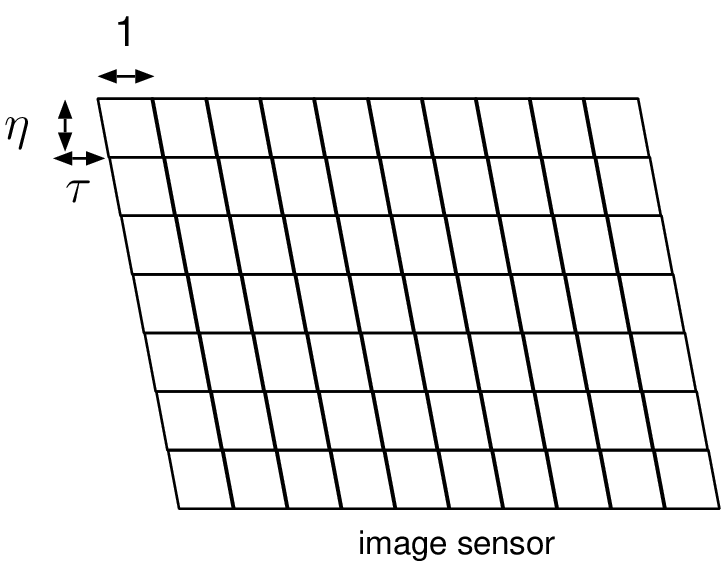
2.3 (b) Non-ideal image sensor with non-square, skewed pixels.
D. Radial lens distortion
Real camera lenses typically suffer from non-linear lens distortion. In practice, radial lens distortion causes straight lines to be mapped as curved lines. As seen in Figure 2.4, the radial lens distortion appears more visible at the image edges, where the radial distance is high. A standard technique to model the radial lens can be described as follows.

2.3 (a) The image \((x,y)\) and camera \((u,v)\) coordinate system. 2.3 (b) Non-ideal image sensor with non-square, skewed pixels.
Let \((x_u,y_u)^T\) and \((x_d,y_d)^T\) be the corrected and the measured distorted pixel positions, respectively. The relation between an undistorted and distorted pixel can be modeled with a polynomial function and can be written as \[\left( \begin{array}{c} x_u-o_x\\ y_u-o_y \end{array} \right) = L(r_d) \left( \begin{array}{c} x_d-o_x\\ y_d-o_y \end{array} \right), \ (2.8)\] where \[L(r_d) = 1 + k_1 r_d^2 \textrm{ }\textrm{ and } \textrm{ } r_d^2 = (x_d-o_x)^2+(y_d-o_y)^2. \ (2.9) \label{eq:radial11}\] In the case \(k_1=0\), it can be noted that \(x_u=x_d\) and \(y_u=y_d\), which corresponds to the absence of radial lens distortion.
It should be noted that Equation (2.8) provides the correct pixel position using a function of the distorted pixel position. However, to generate an undistorted image, it would be more convenient to base the function \(L(r)\) on the undistorted pixel position. This technique is usually known as the inverse mapping method. The inverse mapping technique consists of scanning each pixel in the output image and re-sampling and interpolating the correct pixel from the input image. To perform an inverse mapping, the inversion of the radial lens distortion model is necessary and can be described as follows. First, similar to the second part of Equation (2.9), we define \[r_u^2=(x_u-o_x)^2+(y_u-o_y)^2 (2.10).\] Then, taking the norm of Equation (2.8), it can be derived that \[(x_u-o_x)^2+(y_u-o_y)^2 = L(r_d) \cdot \Big( (x_d-o_x)^2+(y_d-o_y)^2 \Big), (2.11)\] which is equivalent to \[r_u=L(r_d)\cdot r_d. (2.12) \label{eq:radial2}\] When taking into account Equation (2.9), this equation can be rewritten as a cubic polynomial: \[r_d^3+\frac{1}{k_1}r_d-\frac{r_u}{k_1}=0. (2.13) \label{eq:radial3}\] The inverted lens distortion function can be derived by substituting Equation (2.12) into Equation (2.8) and developing it from the right-hand side: \[\left( \begin{array}{c} x_d-o_x\\ y_d-o_y \end{array} \right) = \frac{r_d}{r_u} \left( \begin{array}{c} x_u-o_x\\ y_u-o_y \end{array} \right), (2.14) \label{eq:radial4}\] where \(r_d\) can be calculated by solving the cubic polynomial function of Equation (2.13). This polynomial can be solved using Cardano’s method, by first calculating the discriminant \(\Delta\) defined as \(\Delta = q^2 + 4/27 p^3\) where \(p=1/k_1\) and \(q=-r_u/k_1\). Depending on the sign of the discriminant, three sets of solutions are possible.
If \(\Delta>0\), then the equation has one real root \(r_{d1}\) defined as \[r_{d1} = \sqrt[3]{\frac{-q + \sqrt{\Delta}}{2}} + \sqrt[3]{\frac{-q - \sqrt{\Delta}}{2}}. (2.15)\]
If \(\Delta<0\), then the equation has three real roots \(r_{dk}\) defined by \[r_{dk} = 2 \sqrt{\frac{-p}{3}} \cos{\left(\frac{\arccos(\frac{-q}{2}\sqrt{\frac{27}{-p^3} })+2k\pi}{3}\right)}, (2.16) \] for \(k=\{0,1,2\}\), where an appropriate solution \(r_{dk}\) should be selected such that \(r_{dk}>0\) and \(r_{dk}<r_{uk}\). However, only one single radius corresponds to the practical solution. Therefore, the second case \(\Delta<0\) should not be encountered. The third case with \(\Delta=0\) is also impractical. In practice, we have noticed that, indeed, these second and third cases never occur.
As an example, Figure 2.5 depicts a distorted image and the corresponding corrected image using the inverted mapping method, with \(\Delta>0\).

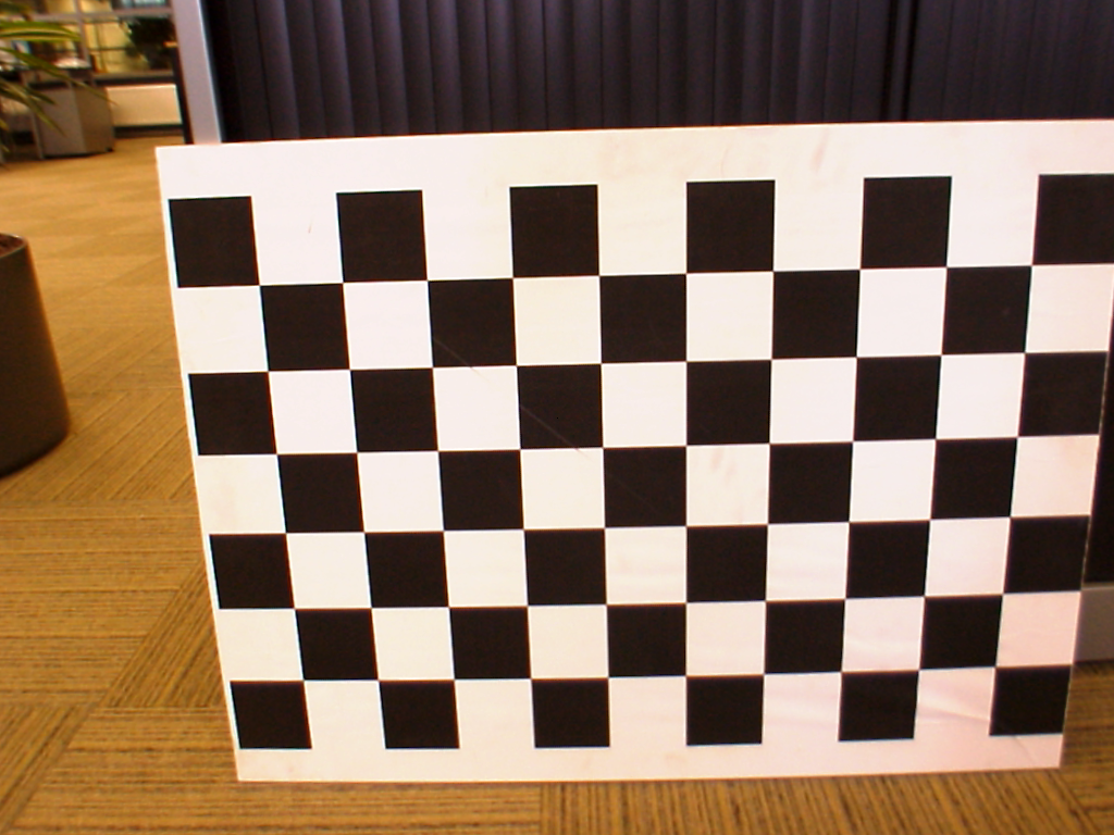
Figure 2.5 (a) Distorted image. (b) Corresponding corrected image using the inverted mapping method.
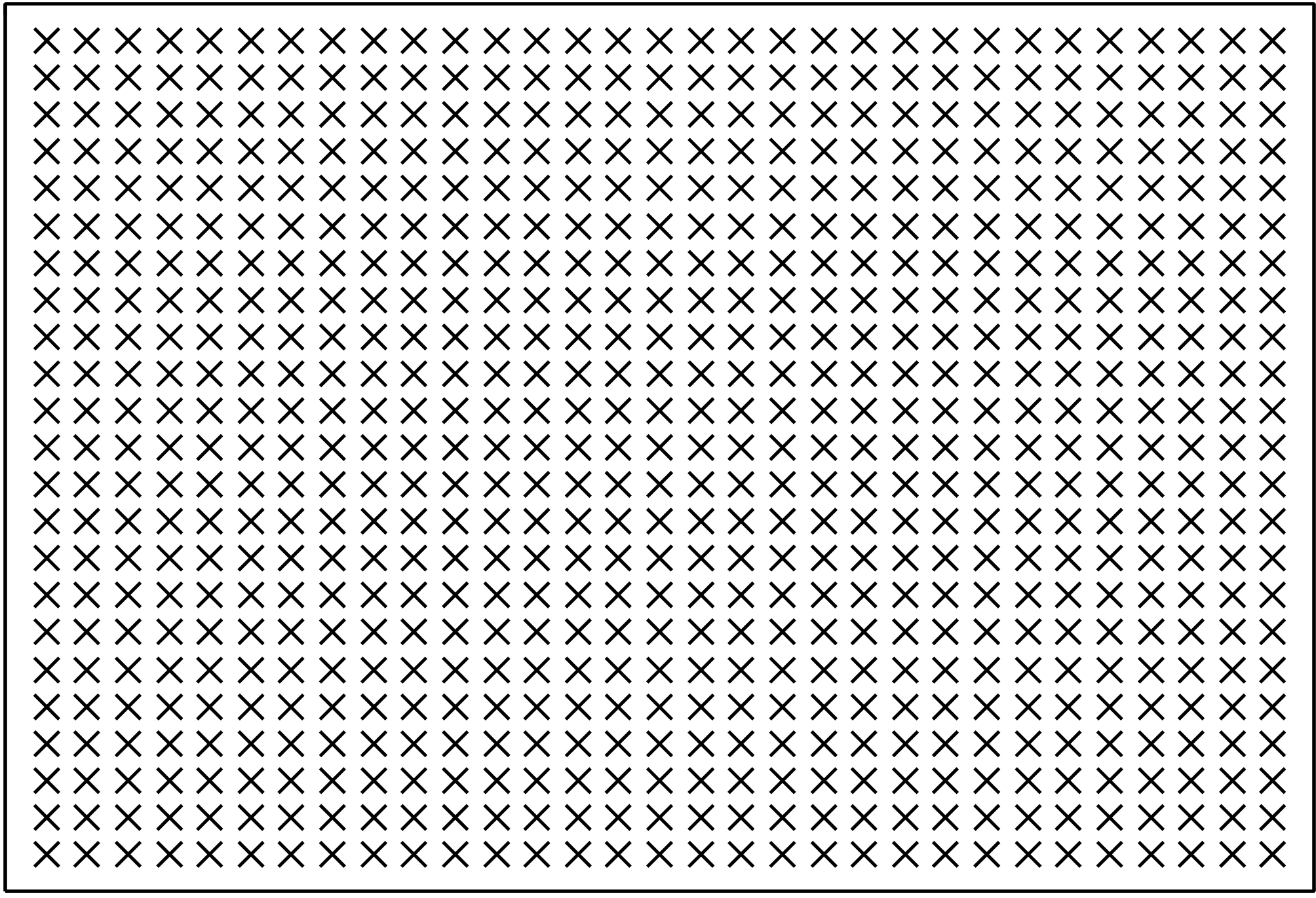
Estimation of the distortion parameters The discussed lens-distortion correction method requires knowledge of the lens parameters, i.e., \(k_1\) and \((o_x,o_y)^T\). The estimation of the distortion parameters can be performed by minimizing a cost function that measures the curvature of lines in the distorted image. To measure this curvature, a practical solution is to detect feature points belonging to the same line on a calibration rig, e.g., a checkerboard calibration pattern (see Figure 2.5). Each point belonging to the same line in the distorted image forms a bended line instead of a straight line [31]. By comparing the deviation of the bended line from the theoretical straight line model, the distortion parameters can be calculated.
Extrinsic parameters
As opposed to the intrinsic parameters that describe internal parameters of the camera (focal distance, radial lens parameters), the extrinsic parameters indicate the external position and orientation of the camera in the 3D world. Mathematically, the position and orientation of the camera is defined by a \(3 \times 1\) vector \(\boldsymbol{C}\) and by a \(3 \times 3\) rotation matrix \(\boldsymbol{R}\) (see Figure [fig:extrinsic_param]).

Figure 2.6 The relationship between the camera and world coordinate system is defined by the camera center \(\boldsymbol{C}\) and the rotation \(\boldsymbol{R}\) of the camera.
To obtain the pixel position \(\boldsymbol{p}=(x,y,1)^T\) of a 3D-world homogeneous point \(\boldsymbol{P}\), the camera should be first translated to the world coordinate origin and second, rotated. This can be mathematically written as \[\lambda \boldsymbol{p} = \left[\boldsymbol{K} | \boldsymbol{0}_3\right] \left[ \begin{array}{cc} \boldsymbol{R} & 0 \\ \boldsymbol{0}_3 & 1 \end{array} \right] \left[ \begin{array}{cc} \boldsymbol{0}_3^T &\boldsymbol{-C} \\ 0 & 1 \end{array} \right] \boldsymbol{P}. (2.17)\] Alternatively, when combining matrices, Equation (2.17) can be reformulated as \[\lambda \boldsymbol{p} = \left[\boldsymbol{K} | \boldsymbol{0}_3\right] \left[ \begin{array}{cc} \boldsymbol{R} & -\boldsymbol{RC} \\ \boldsymbol{0}_3^T & 1 \end{array} \right] \boldsymbol{P} = \boldsymbol{K}\boldsymbol{R} \left( \begin{array}{c} X\\ Y\\ Z \end{array} \right) - \boldsymbol{K}\boldsymbol{R C}. (2.18)\]
Back-projection of a 2D point to 3D
Previously, the process of projecting a 3D point onto the 2D image plane was described. We now present how a 2D point can be back-projected to the 3D space and derive the corresponding coordinates. Considering a 2D point \(\boldsymbol{p}\) in an image, there exists a collection of 3D points that are mapped and projected onto the same point \(\boldsymbol{p}\). This collection of 3D points constitutes a ray connecting the camera center \(\boldsymbol{C}=(C_x,C_y,C_z)^T\) and \(\boldsymbol{p}=(x,y,1)^T\). From Equation (2.18), the ray \(\boldsymbol{P}(\lambda)\) associated to a pixel \(\boldsymbol{p}=(x,y,1)^T\) can be defined as \[\left( \begin{array}{c} X\\ Y\\ Z \end{array} \right) = \underbrace{\boldsymbol{C}+\lambda \boldsymbol{R}^{-1}\boldsymbol{K}^{-1}\boldsymbol{p}} _{ray\ \boldsymbol{P}(\lambda)}, (2.19)\] where \(\lambda\) is the positive scaling factor defining the position of the 3D point on the ray. In the case \(Z\) is known, it is possible to obtain the coordinates \(X\) and \(Y\) by calculating \(\lambda\) using the relation \[\lambda=\frac{Z-C_z}{z_3} \textrm{ where } (z_1,z_2,z_3)^T=\boldsymbol{R}^{-1}\boldsymbol{K}^{-1}\boldsymbol{p}. (2.20)\] The back-projection operation is important for depth estimation and image rendering, which will be extensively addressed later in this thesis. For depth estimation, this would mean that an assumption is made for the value of \(Z\) and the corresponding 3D point is calculated. With an iterative procedure, an appropriate depth value is selected from a set of assumed depth candidates.
Coordinate system conversion
Sometimes, coordinate systems need to be converted to obtain a more efficient computation procedure. Let us now propose two methods that transform the projection matrix, so that new coordinate systems can be employed. We will also provide applications of those methods.
A. Changing the image coordinate system
The definition of the coordinate system in 3D image processing is not uniformly chosen. For example, the calibration parameters of the MPEG test sequences “Breakdancers” and “Ballet” [32] assume a left-handed coordinate system. However, a righ-handed coordinate system is usually employed in literature. Therefore, we outline a method for converting the image coordinate system.
Typically, pixel coordinates are defined such that the origin of the 2D image coordinate system is located at the top left of the image. In this case, the \(x\) and \(y\) axis point horizontally to the right and vertically downward, respectively (convention 1). However, an alternative convention is to locate the origin of the image coordinate system at the bottom left, with the \(y\) image axis pointing vertically upwards. To transform the image coordinate system, it is necessary to flip the \(y\) image axis and translate the origin along the \(y\) image axis. This can be performed using the matrix denoted \(\boldsymbol{B}_1\) (see Equation (2.21)). Additionally, one can distinguish two possible conventions for defining the orientation of the 3D world axis: either a left-handed or a right-handed coordinate system can be adopted. The conversion of a left-handed to a right-handed coordinate system can be performed by flipping the \(Y\) world axis 3 (matrix \(\boldsymbol{B}_2\)). By concatenating the two conversion matrices \(\boldsymbol{B}_1\) and \(\boldsymbol{B}_2\) with the original projection matrix, one can obtain the converted projection matrix \[\lambda \boldsymbol{p} = \underbrace{ \underbrace{ \left( \begin{array}{ccc} 1&0&0\\ 0&-1&h-1\\ 0&0&1\\ \end{array} \right) } _{\boldsymbol{B}_1} \left[K | \boldsymbol{0}_3\right] \left[ \begin{array}{cc} \boldsymbol{R} & -\boldsymbol{R}\boldsymbol{C} \\ 0 & 1 \end{array} \right] \underbrace{ \left( \begin{array}{cccc} 1&0&0&0\\ 0&-1&0&0\\ 0&0&1&0\\ 0&0&0&1\\ \end{array} \right) } _{\boldsymbol{B}_2} } _{\textrm{converted projection matrix }} \boldsymbol{P}, (2.21)\] where \(h\) corresponds to the height of the image. The obtained converted projection matrix is then defined in an image coordinate system using the convention 1 notation and in a right-handed world coordinate system. Finally, it should be noted that the conversion of the image coordinate system is achieved by modifying the intrinsic parameters while the conversion of the world coordinate system is made by transforming the extrinsic parameters. This is the reason why conversion matrices \(\boldsymbol{B}_1\) and \(\boldsymbol{B}_2\) are placed as left and right terms in Equation (2.21).
B. Changing the world coordinate system
A conversion is used for re-specifying depth images into a new world coordinate system. This conversion involves the calculation of the position of a 3D point specified in another camera coordinate system and the projection of this 3D point onto the other image plane. The modification of the location and orientation of the world coordinate system is performed in a way similar to the above-described method. Figure 2.7 illustrates the definition of two world coordinate systems.
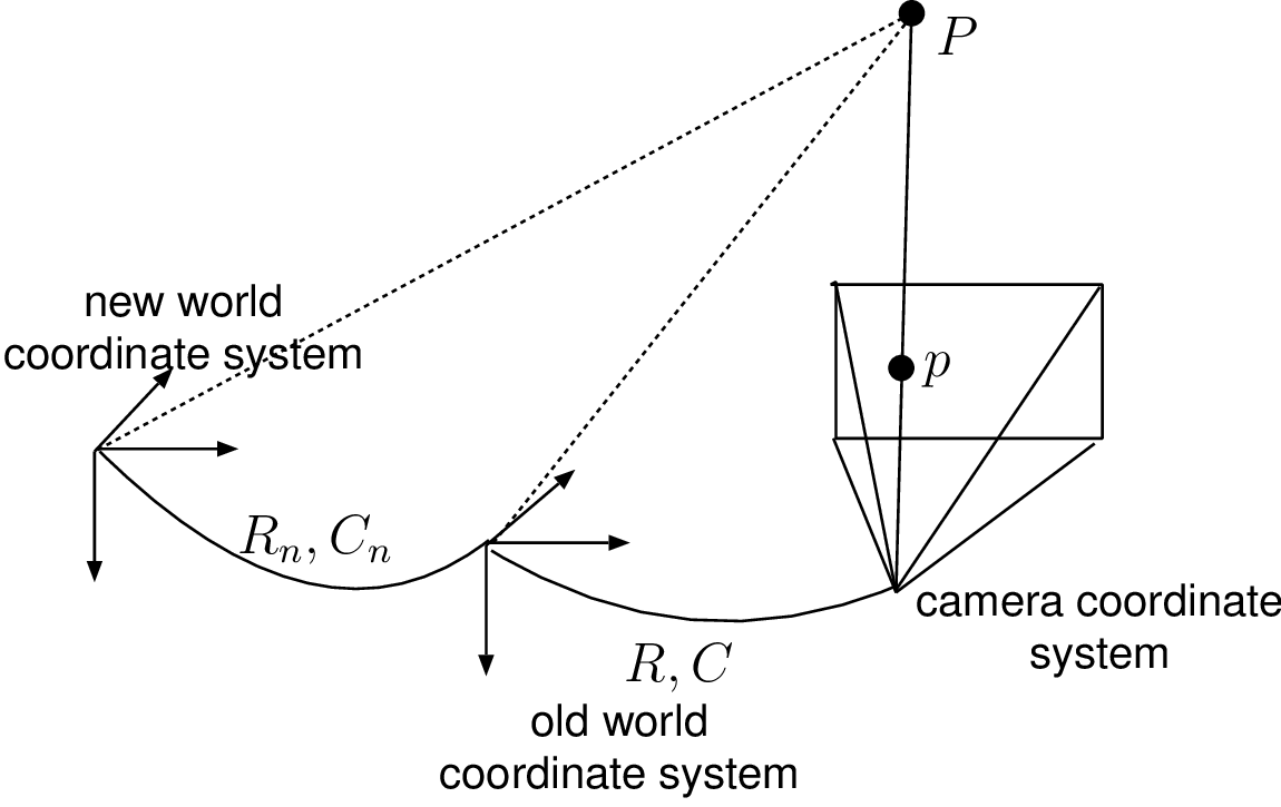
Figure 2.7 A 3D point \(\boldsymbol{P}\) can be defined in two different world coordinate systems. Defining \(\boldsymbol{P}\) in a new coordinate system involves (1) the conversion of its 3D coordinates and (2) the conversion of the extrinsic parameters.
The modification of the world coordinate system involves the simultaneous conversion of the projection matrix and the coordinates of the 3D point. Considering a 3D world point \(\boldsymbol{P}\) and a camera defined with a projection matrix with intrinsic and extrinsic parameters \(\boldsymbol{K}\), \(\boldsymbol{R}\) and \(\boldsymbol{C}\), the coordinate-system conversion can be carried out in two steps. First, specify the projection matrix in a new world coordinate system, where only the position and orientation of the camera, i.e., extrinsic parameters, should be modified. The extrinsic parameters are converted using the position \(\boldsymbol{C}_n\) and orientation \(\boldsymbol{R}_n\) of the new coordinate system defined, with respect to the original coordinate system. Second, specify the position of a 3D point \(\boldsymbol{P}\) in the new coordinate system. The coordinate-system conversion can be written as \[\begin{aligned} \lambda \boldsymbol{p} = \left[ \boldsymbol{K} | \boldsymbol{0}_3 \right] \underbrace{ \left[ \begin{array}{cc} \boldsymbol{R }& \boldsymbol{-R C} \\ \boldsymbol{0}_3^T & 1 \end{array} \right] \left[ \begin{array}{cc} \boldsymbol{R}_n^T & \boldsymbol{C}_n \\ \boldsymbol{0}_3^T & 1 \end{array} \right] } _{\textrm{converted extrinsic parameters}} \underbrace { \left[ \begin{array}{cc} \boldsymbol{R}_n & \boldsymbol{-R}_n \boldsymbol{C}_n \\ \boldsymbol{0}_3^T & 1 \end{array} \right] \boldsymbol{P}, }_{\textrm{converted 3D position} } (2.22)\end{aligned}\] where \(\boldsymbol{p}\) represents the projected pixel position and the all-zero element vector is denoted by \(\boldsymbol{0}_3\).
Camera calibration
Camera calibration involves the estimation of both extrinsic and intrinsic camera parameters. This section does not present a new calibration algorithm, but instead shortly describes a parameter-estimation technique for calibrating a multi-view camera setup. To compute the camera parameters, a practical technique [33] based on a calibration rig is employed. As for correcting the lens distortion, the estimation of camera parameters is based on a calibration rig with known geometry, such as a checkerboard pattern. Using various perspective views of the checkerboard, the algorithm estimates the position, orientation and internal parameters of the camera. The process of estimating all camera parameters is known as strong calibration, which will be addressed in the sequel.
Camera parameters estimation
Let us consider a planar checkerboard that defines a right-handed 3D world coordinate system (see Figure 2.8). The first stage of the camera calibration procedure is to establish correspondences between 2D points in the image and 3D points on the checkerboard, i.e., so-called point-correspondences. In practice, a robust extraction of point-correspondences can be performed by exploiting the topological structure of the checkerboard pattern [34].
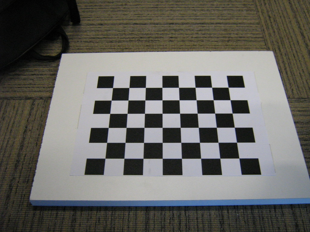
A planar checkerboard pattern defines a 3D world coordinate system, and additionally enables the detection of 3D feature points.
Because each 3D feature point belongs to the board plane \(Z=0\), the projection of each 2D point onto the image plane can be written as \[\lambda \left( \begin{array}{c} x\\ y\\ 1 \end{array} \right) = \left[K | \boldsymbol{0}_3\right] \left[ \begin{array}{cc} \boldsymbol{R} & -\boldsymbol{R}\boldsymbol{C} \\ \boldsymbol{0}_3^T & 1 \end{array} \right] \left( \begin{array}{c} X\\ Y\\ Z=0\\ 1 \end{array} \right), (2.23)\] which can be reformulated to \[\lambda \left( \begin{array}{c} x\\ y\\ 1 \end{array} \right) = \underbrace{ \boldsymbol{K} \left[\ \boldsymbol{r}_1\ \boldsymbol{r}_2\ \boldsymbol{t}\ \right] } _{\text{homography transform}\ \boldsymbol{H}} \left( \begin{array}{c} X\\ Y\\ 1 \end{array} \right), (2.24)\] where \(\boldsymbol{r}_{i}\) corresponds to the \(i^{th}\) column of the rotation matrix \(\boldsymbol{R}\) and \(\boldsymbol{t}=-\boldsymbol{RC}\). Because the matrix product \(\boldsymbol{K}\left[\ \boldsymbol{r}_1\ \boldsymbol{r}_2\ \boldsymbol{t}\ \right]\) is a \(3 \times 3\) matrix, it corresponds to a so-called planar homography transform, which is typically denoted as a matrix \(\boldsymbol{H}\). A planar homography transform is a non-singular linear relation between two planes [35]. In our case, the homography transform defines a linear mapping of points between the planar checkerboard (3D position) and the image plane (pixel position). The calculation of the camera parameters requires the estimation of the homography transform \(\boldsymbol{H}\): \[\lambda \left( \begin{array}{c} x\\ y\\ 1 \end{array} \right) = \underbrace{ \left( \begin{array}{ccc} h_{11} &h_{12} &h_{13} \\ h_{21} &h_{22} &h_{23} \\ h_{31} &h_{32} &h_{33} \end{array} \right) }_{homography\ \boldsymbol{H}} \left( \begin{array}{c} X\\ Y\\ 1 \end{array} \right). (2.25)\]
A. Homography transform estimation
The homography \(\boldsymbol{H}\) can be estimated by detecting point-correspondences \(\boldsymbol{p}_i \leftrightarrow \boldsymbol{P}_i'\) with \(\boldsymbol{p}_i=(x_i,y_i,1)^T\) being the pixel position and \(\boldsymbol{P}_i'=(X_{i},Y_{i},1)^T\) being the world coordinates of the corresponding feature point of index \(i\) on the checkerboard. Using the previously introduced notation, Equation (2.25) may be written as \[\lambda \boldsymbol{p}_i = \boldsymbol{H} \boldsymbol{P}_i' (2.26)\]
In order to eliminate the scaling factor, one can calculate the cross product of each term of Equation (2.26), leading to \[\boldsymbol{p}_i \times (\lambda \boldsymbol{p}_i )= \boldsymbol{p}_i \times ( \boldsymbol{H} \boldsymbol{P}_i'), (2.27)\] and since \( \boldsymbol{p}_i \times \boldsymbol{p}_i=\boldsymbol{0}_3\), Equation (2.27) may be written as \[\boldsymbol{p}_i \times \boldsymbol{H} \boldsymbol{P}_i' =\boldsymbol{0}_3. (2.28)\] Writing the matrix product \(\boldsymbol{H} \boldsymbol{P}_i'\) as \[\boldsymbol{H} \boldsymbol{P}_i'= \left[ \begin{array}{c} \boldsymbol{h}^{1T} \boldsymbol{P}_i' \\ \boldsymbol{h}^{2T} \boldsymbol{P}_i'\\ \boldsymbol{h}^{3T} \boldsymbol{P}_i' \end{array} \right] , (2.29)\] with \(\boldsymbol{h}^{mT}\) being the transpose 4 of the \(m-th\) row of \(\boldsymbol{H}\), we rework Equation (2.28) into \[\boldsymbol{p}_i\times \boldsymbol{H} \boldsymbol{P}_i' = \left( \begin{array}{c} x_i\\ y_i\\ 1 \end{array} \right) \times \left[ \begin{array}{c} \boldsymbol{h}^{1T} \boldsymbol{P}_i' \\ \boldsymbol{h}^{2T} \boldsymbol{P}_i'\\ \boldsymbol{h}^{3T} \boldsymbol{P}_i' \end{array} \right] = \left[ \begin{array}{c} y_i \boldsymbol{h^{3T}} \boldsymbol{P}_i' - \boldsymbol{h^{2T}} \boldsymbol{P}_i' \\ \boldsymbol{h^{1T}} \boldsymbol{P}_i' - x_i \boldsymbol{h^{3T}} \boldsymbol{P}_i' \\ x_i \boldsymbol{ h^{2T}} \boldsymbol{P}_i' - y_i \boldsymbol{h^{1T}} \boldsymbol{P}_i' \end{array} \right] =\boldsymbol{0}_3. (2.30)\] Since Equation (2.30) is linear in \(\boldsymbol{h}^{mT}\) and noting that \(\boldsymbol{h}^{mT} \boldsymbol{P}_i'\) \(=\boldsymbol{P}_{i}^{'T} \boldsymbol{h}^m \), Equation (2.30) may be reformulated as \[\left[ \begin{array}{ccc} \boldsymbol{0}_3^T & -\boldsymbol{P}_i^{'T} & y_i \boldsymbol{P}_i^{'T} \\ \boldsymbol{P}_i^{'T} & \boldsymbol{0}_3^T & -x_i \boldsymbol{P}_i^{'T} \\ -y_i \boldsymbol{P}_i^{'T} & x_i\boldsymbol{P}_i^{'T} & \boldsymbol{0}_3^T \end{array} \right] \left[ \begin{array}{c} \boldsymbol{ h}^{1}\\ \boldsymbol{ h}^{2}\\ \boldsymbol{ h}^{3} \end{array} \right] =\boldsymbol{0}_9. (2.31)\] Note that the rows of the previous matrix are not linearly independent: the third row is the sum of \(-x_i\) times the first row and \(-y_i\) times the second row. Thus, for each point-correspondence, Equation (2.31) provides two linearly independent equations. The two first rows are typically used for solving \(\boldsymbol{H}\). Because the homography transform is written using homogeneous coordinates, the homography \(\boldsymbol{H}\) is defined using \(8\) parameters plus a free \(9^{th}\) homogeneous scaling factor. Therefore, at least \(4\) point-correspondences providing \(8\) equations are required to compute the homography. Practically, a larger number of correspondences is employed so that an over-determined linear system is obtained. By rewriting \(\boldsymbol{H}\) in a vector form as \(\boldsymbol{h}=[h_{11},h_{12},h_{13},h_{21},h_{22},h_{23},h_{31},h_{32},h_{33}]^T\), \(n\) pairs of point-correspondences enable the construction of a \(2n \times 9\) linear system, which is expressed by (\(i\) corresponds to the index of the feature point, hence \(i=1\) for first two rows, \(i=2\) for the second two rows, etc.) \[\underbrace{ \left( \begin{array}{ccccccccc} 0 &0 &0 & -X_1 & -Y_1 &-1 & y_1 X_1 & y_1 X_1 & y_1 \\ X_1 & Y_1 &1 & 0 &0 &0 & -x_1 X_1 & -x_1 Y_1 & -x_1 \\ 0 &0 &0 & -X_2 & -Y_2 &-1 & y_2 X_2 & y_2 X_2 & y_2 \\ X_2 & Y_2 &1 & 0 &0 &0 & -x_2 X_2 & -x_2 Y_2 & -x_2 \\ \vdots &\vdots &\vdots &\vdots &\vdots &\vdots &\vdots &\vdots &\vdots \\ 0 &0 &0 & -X_n & -Y_n &-1 & y_n X_n & y_n X_n & y_n \\ X_n & Y_n &1 & 0 &0 &0 & -x_n X_n & -x_n Y_n & -x_n \\ \end{array} \right) }_{\boldsymbol{C}} \left( \begin{array}{c} h_{11}\\ h_{12}\\ h_{13}\\ h_{21}\\ h_{22}\\ h_{23}\\ h_{31}\\ h_{32}\\ h_{33} \end{array} \right) =\boldsymbol{0_9}. (2.32)\] Solving this linear system involves the calculation of a Singular Value Decomposition (SVD). Such an SVD corresponds to reworking the matrix to the form of the matrix product \(\boldsymbol{C}=\boldsymbol{UDV^T}\), where the solution \(\boldsymbol{h}\) corresponds to the last column of the matrix \(\boldsymbol{V}\). To avoid numerical instabilities, the coordinates of point-correspondences should be normalized. This technique is known as the normalized Direct Linear Transformation (DLT) algorithm [35]. It should be noted that a non-linear refinement of the solution may be performed afterwards. However, such a non-linear refinement does not yield a significant improvement and moreover, it involves the calculation of a Jacobian matrix, required for the non-linear Levenberg-Marquardt optimization.
B. Calculation of intrinsic parameters
Assuming that the homography transform \(\boldsymbol{H}\) is calculated, the intrinsic parameters can be recovered using the a-priori knowledge that \(\boldsymbol{r}_1\) and \(\boldsymbol{r}_2\) are orthonormal. Denoting the homography transform as \(\boldsymbol{H}=[\boldsymbol{h}_1\ \boldsymbol{h}_2\ \boldsymbol{h}_3]\), it can be derived from Equation (2.24) that \([\boldsymbol{h}_1\ \boldsymbol{h}_2] = \lambda' \boldsymbol{K}\cdot[\boldsymbol{r}_1\ \boldsymbol{r}_2]\) which is equivalent to \( \boldsymbol{K}^{-1}\cdot [\boldsymbol{h}_1\ \boldsymbol{h}_2] = \lambda' [\boldsymbol{r}_1\ \boldsymbol{r}_2]\), where \(\lambda'\) is a homogeneous factor. Assuming that the vectors \(\boldsymbol{r}_1\), \(\boldsymbol{r}_2\) of the rotation matrix \(\boldsymbol{R}\) are orthonormal, then the vectors \(\boldsymbol{r}_1\) and \(\boldsymbol{r}_2\) are perpendicular to each other and have equal norm 5, so that \[\begin{array}{l} (\boldsymbol{h}_1^T \boldsymbol{K}^{-T} \cdot \boldsymbol{K}^{-1}\boldsymbol{h}_2 ) = 0 , \\ \boldsymbol{h}_1^T \boldsymbol{K}^{-T} \cdot \boldsymbol{K}^{-1}\boldsymbol{h}_1 = \boldsymbol{h}_2^T \boldsymbol{K}^{-T} \cdot \boldsymbol{K}^{-1}\boldsymbol{h}_2 . (2.33) \end{array}\] The internal term \(\boldsymbol{K}^{-T}\boldsymbol{K}^{-1}\) appears regularly, which for further use is defined as \(\boldsymbol{B}\) and can be written as \[\begin{array}{ll} \boldsymbol{B}=\boldsymbol{K}^{-T}\boldsymbol{K}^{-1}= \left( \begin{array}{ccc} B_{11} &B_{12} &B_{13}\\ B_{12} &B_{22} &B_{23}\\ B_{13} &B_{23} &B_{33} \end{array} \right) & \\ =\left( \begin{array}{ccc} \frac{1}{\alpha^2} & - \frac{\gamma}{\alpha^2\beta} & \frac{\gamma o_y-\beta o_x}{\alpha^2 \beta} \\ -\frac{\gamma}{\alpha^2\beta} & \frac{\gamma^2+\alpha^2}{\alpha^2\beta^2} & \frac{(-\gamma^2-\alpha^2)o_y+ \beta \gamma o_x}{\alpha^2 \beta^2} \\ \frac{\gamma o_y - \beta o_x}{\alpha^2 \beta} & \frac{(-\gamma^2-\alpha^2)o_y+ \beta \gamma o_x}{\alpha^2 \beta^2}& \frac{(\gamma^2+\alpha^2)o_y^2-2\beta \gamma o_x o_y+\beta^2 o_y^2+\alpha^2 \beta^2}{\alpha^2 \beta^2} \end{array} \right). & \end{array} (2.34)\] This matrix covers the intrinsic parameters of the camera, such as the focal length \(\alpha=f\), aspect-ratio related parameter \(\beta=\eta f\) and skew \(\gamma= \tau\). This description corresponds to the notation adopted in the literature [33]. By writing \(\boldsymbol{B}\) in a vector form and omitting the double terms from the symmetry in \(\boldsymbol{B}\), we find a reduced vector \(\boldsymbol{b}\) with only 6 terms, thus \(\boldsymbol{b}=[B_{11},B_{12},B_{22},B_{13},B_{23},B_{33}]^T\). Referring to Equation (2.33), and starting with the bottom equation and generalizing it with the difference in index in the top equation, we can write the general expression of \(\boldsymbol{h}_k^{T}\boldsymbol{B}\boldsymbol{h}_l\) as \[\boldsymbol{h}_k^{T} \boldsymbol{B} \boldsymbol{h}_l=\boldsymbol{v}_{kl}^T\boldsymbol{b}, (2.35)\] with \[\begin{array}{ll} \boldsymbol{v}_{kl}=&[h_{k1}h_{l1}, h_{k1} h_{l2}+h_{k2} h_{l1},h_{k2}h_{l2}, \\ &h_{k3}h_{l1}+h_{k1}h_{l3},h_{k3}h_{l2}+h_{k2}h_{l3},h_{k3}h_{l3}]^T, \end{array} (2.36)\] and \(\boldsymbol{h}_k\) being the \(k^{th}\) column vector of \(\boldsymbol{H}\) with \(\boldsymbol{h}_k=[h_{k1},h_{k2},h_{k3}]^T\). For each homography or image of the checkerboard, Equation (2.33) can be written as \[\left[ \begin{array}{c} \boldsymbol{v}_{12}^T\\ (\boldsymbol{v}_{11}-\boldsymbol{v}_{22})^T \end{array} \right] \boldsymbol{b}=0. (2.37)\] Note that the vector \(\boldsymbol{b}\) which summarizes the intrinsic parameters, is a 6-element vector so that 6 equations are necessary to recover all camera parameters. Therefore, since each homography provides 2 linear equations, at least 3 homographies or captured images are sufficient. Assuming that \(n\) homography transforms are known, the linear system composed of \(n\) instances of Equation (2.37) can be written as \[\boldsymbol{Vb}=\boldsymbol{0}, (2.38)\] with \(\boldsymbol{V}\) referring to a \(2 n \times 6\) matrix. This linear system can be solved by employing the standard technique of Singular Value Decomposition. Using the computed solution vector \(\boldsymbol{b}\), the intrinsic parameters can be derived [33] as follows. The computed vector \(\boldsymbol{b}=[B_{11},B_{12},B_{22},B_{13},B_{23},B_{33}]^T\) is expanded into the symmetric matrix \(\boldsymbol{B}\), by inserting again the omitted symmetric matrix elements. Rewriting the matrix \(\boldsymbol{B}\) as \(\boldsymbol{B}=\lambda \boldsymbol{K}^{-T} \boldsymbol{K}^{-1}\) (Equation 2.34), we finally find the intrinsic parameters as \[\begin{array}{l} o_y=\frac{(B_{12}B_{13}-B_{11}B_{23})}{B_{11}B_{22}-B_{12}^2},\\ \lambda= B_{33}-\frac{B_{13}^2+o_y(B_{12}B_{13}-B_{11}B_{23})}{B_{11}},\\ \alpha=\sqrt{\frac{\lambda}{B_{11}}},\\ \beta=\sqrt{\frac{\lambda B_{11}}{B_{11}B_{22}-B_{12}^2}},\\ \gamma=\frac{-B_{12}\alpha^2\beta }{\lambda},\\ o_x=\frac{\gamma o_y}{\beta}-\frac{B_{13}\alpha^2}{\lambda}. \end{array} (2.39)\]
C. Calculation of extrinsic parameters
The position and orientation of the camera can be recovered from Equation (2.24) and written as \[\begin{array}{l} \boldsymbol{r}_1=\lambda_1 \boldsymbol{K}^{-1}\boldsymbol{h}_1,\\ \boldsymbol{r}_2=\lambda_2 \boldsymbol{K}^{-1}\boldsymbol{h}_2,\\ \boldsymbol{t}=-\boldsymbol{RC}=\lambda_3 \boldsymbol{K}^{-1}\boldsymbol{h_3}. \end{array} (2.40)\] Given the vectors \(\boldsymbol{r}_1\) and \(\boldsymbol{r}_2\) and bearing in mind that the rotation matrix is orthogonal, the third vector \(\boldsymbol{r}_3\) to complete the matrix \(\boldsymbol{R}\) is found by \[\boldsymbol{r}_3=\boldsymbol{r}_1 \times \boldsymbol{r}_2, (2.41)\] where \(\times\) denotes a cross product. The scaling parameters are calculated by \(\lambda_1=1/ \|\boldsymbol{K}^{-1} \boldsymbol{h}_1 \|\) and \(\lambda_2=1/ \|\boldsymbol{K}^{-1} \boldsymbol{h}_2 \|\) and \(\lambda_3=(\lambda_1+\lambda_2 )/ 2\). Theoretically, we have \(\lambda_1=\lambda_2\). However, due to inaccuracies in the feature-point estimation procedure, both terms may differ and have to be treated separately.
D. Non-linear refinement of the camera parameters
To refine the obtained camera parameters, it is possible to perform a non-linear minimization of a projection function. This function is projecting the 3D points onto the image plane and accumulating the differences between corresponding points. The function is specified by \[\sum_{j}^N \sum_i^n \parallel \boldsymbol{p}_{ij} - \Big( \left[K | \boldsymbol{0}_3 \right] \left[ \begin{array}{cc} \boldsymbol{R}_j & -\boldsymbol{R}_j\boldsymbol{C}_j \\ 0 & 1 \end{array} \right] \boldsymbol{P}_{ij} \Big) \parallel^2, (2.42)\] where \(j\) denotes the image index and \(i\) corresponds to the point-correspondence index.
E. Summary of camera calibration steps
The camera calibration algorithm can be summarized as follows.
Capture \(N\) (at least 3) images with the checkerboard pattern and estimate point-correspondences.
Estimate and correct the radial lens distortion.
For each captured image, calculate the \(N\) homography transforms.
Using the \(N\) homography transforms, calculate the intrinsic and extrinsic parameters.
Refine the calculated camera parameters as explained in Section D above.
As opposed to the standard technique [33], we perform the correction of the non-linear radial lens distortion prior to the camera calibration procedure. This slight modification yields more accurate results for obtaining the homographies \(\boldsymbol{H}_i\) and, afterwards, more accurate calibration parameters.
Two-view geometry
In the previous section, we have described the geometry of a single camera. We now examine the case of two camera views capturing the same scene from two different viewpoints. Given two images, we are interested in estimating the 3D structure of the scene. The estimation of coordinates of a 3D point \(\boldsymbol{P}\) can be performed in two steps. First, given a selected pixel \(\boldsymbol{p}_1\) in the image \(I_1\), the position of the corresponding pixel \(\boldsymbol{p}_2\) in image \(I_2\) is estimated. Similarly to the previous section, a pair of corresponding points \(\boldsymbol{p}_1\) and \(\boldsymbol{p}_2\) is called a point-correspondence. This correspondence in points \(\boldsymbol{p}_1\) and \(\boldsymbol{p}_2\) comes from the projection of the same point \(\boldsymbol{P}\) onto both images \(I_1\) and \(I_2\). Second, the position of \(\boldsymbol{P}\) is calculated by triangulation of the two corresponding points, using the geometry of the two cameras. The geometry of the two cameras relates to the respective position and orientation and internal geometry of each individual camera. The underlying geometry that describes the relationship between both cameras is known as the epipolar geometry. The estimation process of the epipolar geometry is known as weak calibration, as opposed to the strong calibration mentioned earlier in this chapter. The epipolar geometry addresses (among others) the following two aspects.
Geometry of point-correspondence: considering a point in an image, the epipolar geometry provides a constraint on the position of the corresponding point.
Scene geometry: given point-correspondences and the epipolar geometry of both cameras, a description of the scene structure can be recovered.
Epipolar geometry
Let us now describe the geometry of two images and define their mutual relation. Consider a 3D point \(\boldsymbol{P}\) that is projected through the camera centers \(\boldsymbol{C}_1\) and \(\boldsymbol{C}_2\) onto two images at pixel positions \(\boldsymbol{p}_1\) and \(\boldsymbol{p}_2\), respectively (see Figure 2.9(a)).

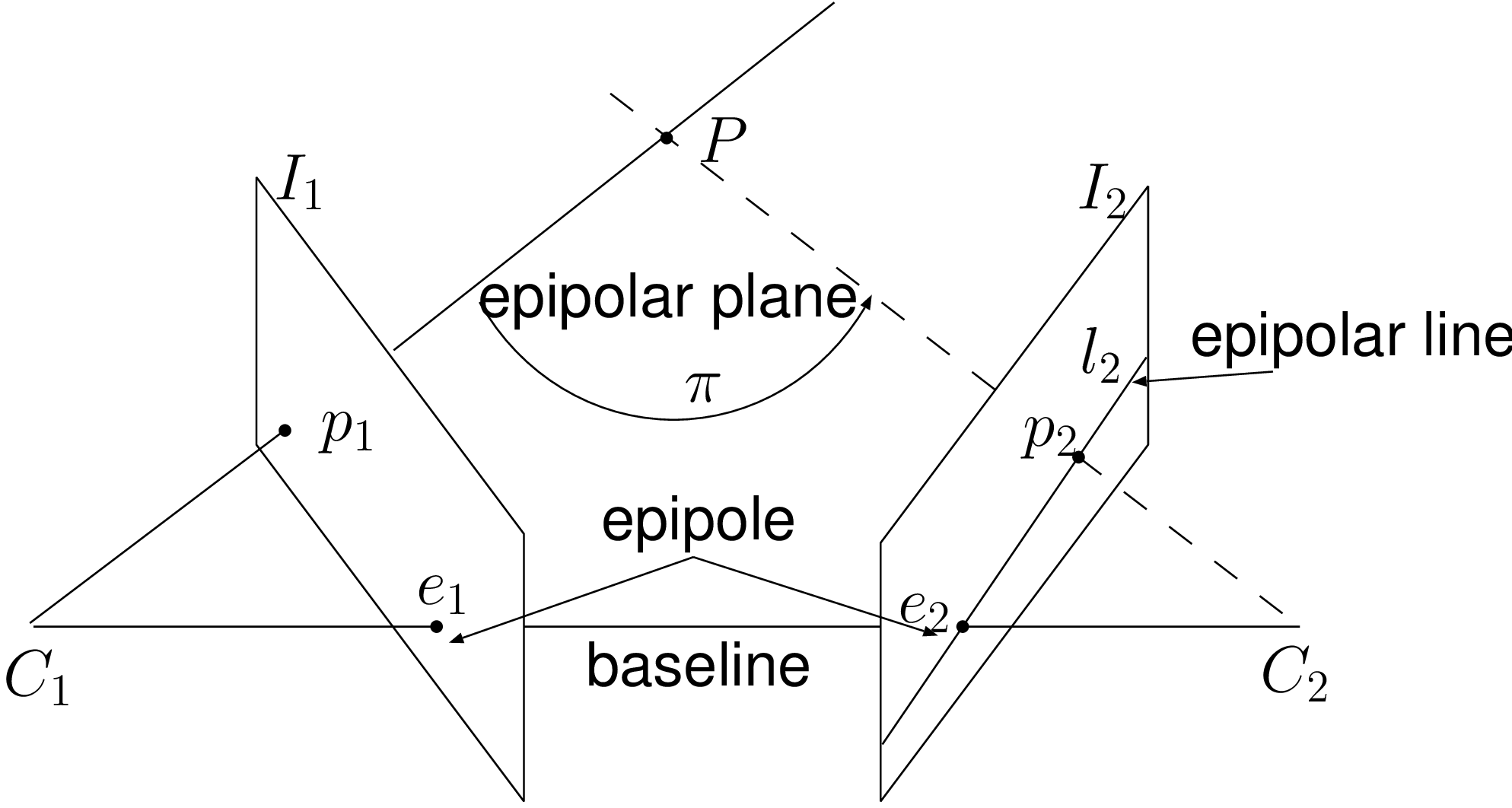
Figure 2.9 Epipolar geometry. (a) The epipolar plane is defined by the point \(\boldsymbol{P}\) and the two camera centers \(\boldsymbol{C}_1\) and \(\boldsymbol{C}_2\). (b) Two cameras and imge planes with an indication of the terminology of epipolar geometry.
Obviously, the 3D points \(\boldsymbol{P}\), \(\boldsymbol{C}_1\), \(\boldsymbol{C}_2\) and the projected points \(\boldsymbol{p}_1\), \(\boldsymbol{p}_2\) are all located within one common plane. This common plane denoted \(\boldsymbol{\pi}\) is known as the epipolar plane. The epipolar plane is fully determined by the back-projected ray going through \(\boldsymbol{C}_1\) and \(\boldsymbol{p}_1\) and the camera center \(\boldsymbol{C}_2\). The property that the previously specified points belong to the epipolar plane provides a constraint for searching point-correspondences. More specifically, considering the image point \(\boldsymbol{p}_1\), a point \(\boldsymbol{p}_2\) lies on the intersection of the plane \(\boldsymbol{\pi}\) with the second image plane (denoted within \(I_2\) in Figure 2.9(a)). The intersection of both planes corresponds to a line known as the epipolar line. Therefore, the search of point-correspondences can be limited to a search along the epipolar line instead of an exhaustive search in the image. Additionally, it is interesting to note that this constraint is independent of the scene structure, but instead, uniquely relies on the epipolar geometry. The epipolar geometry can be described using a \(3\times 3\) rank-\(2\) matrix, called the fundamental matrix \(\boldsymbol{F}\), which is defined by \(\boldsymbol{l_2}=\boldsymbol{F}\boldsymbol{p}_1\). An example of two views with the computed epipolar lines superimposed onto the images is given in Figure 2.10.

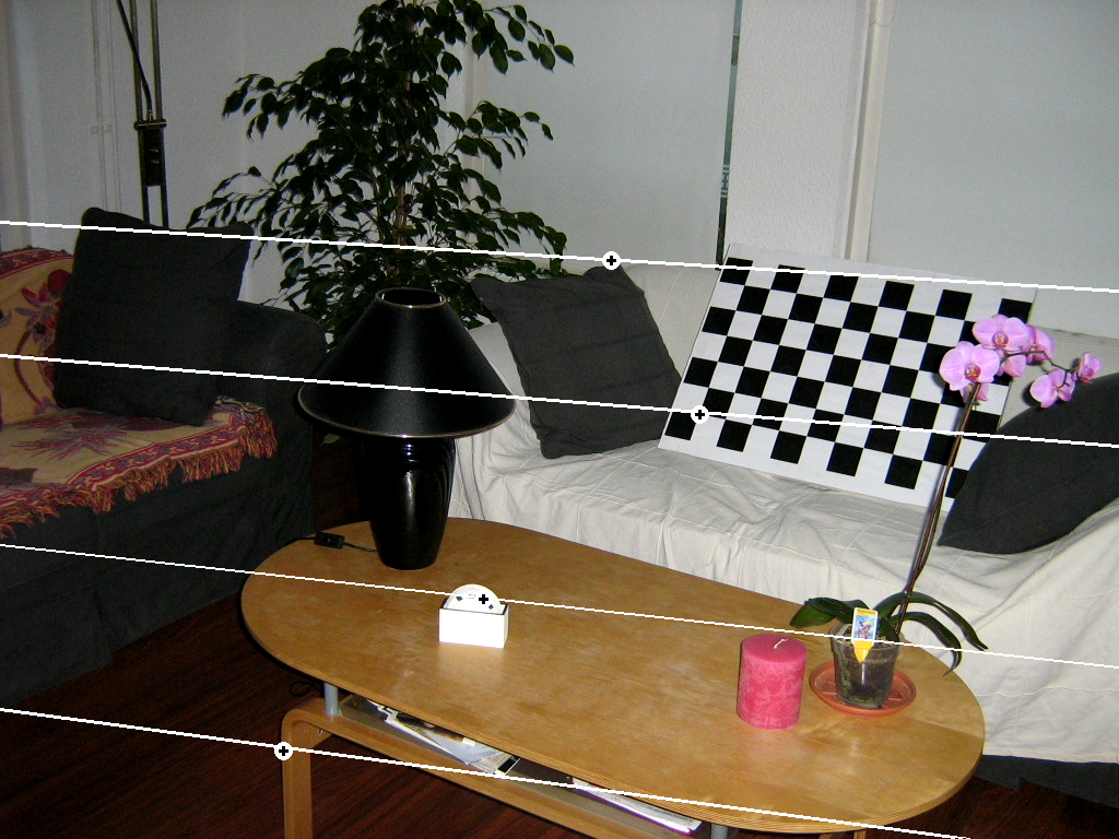
Figure 2.10 Two views of a scene with 4 superimposed epipolar lines.
We now introduce some terminology related to the epipolar geometry employed further in this thesis.
The epipolar plane is the plane defined by a 3D point and the two cameras centers.
The epipolar line is the line determined by the intersection of the image plane with the epipolar plane.
The baseline is the line going through the two cameras centers.
The epipole is the image-point determined by the intersection of the image plane with the baseline. Also, the epipole corresponds to the projection of the first camera center (say \(\boldsymbol{C}_1\)) onto the second image plane (say \(I_2\)), or vice versa.
As previously highlighted, three-dimensional structural information can be extracted from two images by exploiting the epipolar geometry. It was shown that the three-dimensional structure can be extracted by determining the correspondences in the two views and that the point-corresponden-ces can be searched along the epipolar line only. To simplify the search, images are typically captured such that all epipolar lines are parallel and horizontal. In this case, the search of point-correspondences can be performed along the horizontal raster lines of both images. However, it is difficult to accurately align and orient the two cameras such that epipolar lines are parallel and horizontal. Instead, an alternative approach is to capture two views (without alignment and orientation constraints) and transform both images to synthesize two novel views with parallel and horizontal epipolar lines. This procedure is called image rectification which will be described in the next section.
Image rectification
Image rectification is the process of transforming two images \(I_1\) and \(I_2\) such that their epipolar lines are horizontal and parallel. This procedure is particularly useful for depth-estimation algorithms because the search of point-correspondences can be performed along horizontal raster image lines. Practically, the image-rectification operation corresponds to a virtual rotation of two cameras, so that they would become aligned. As illustrated by Figure 2.11, an image-rectification technique [36] consists of synthesizing a common image plane \(I'\) and re-projecting the two images \(I_1\) and \(I_2\) onto this synthetic plane.
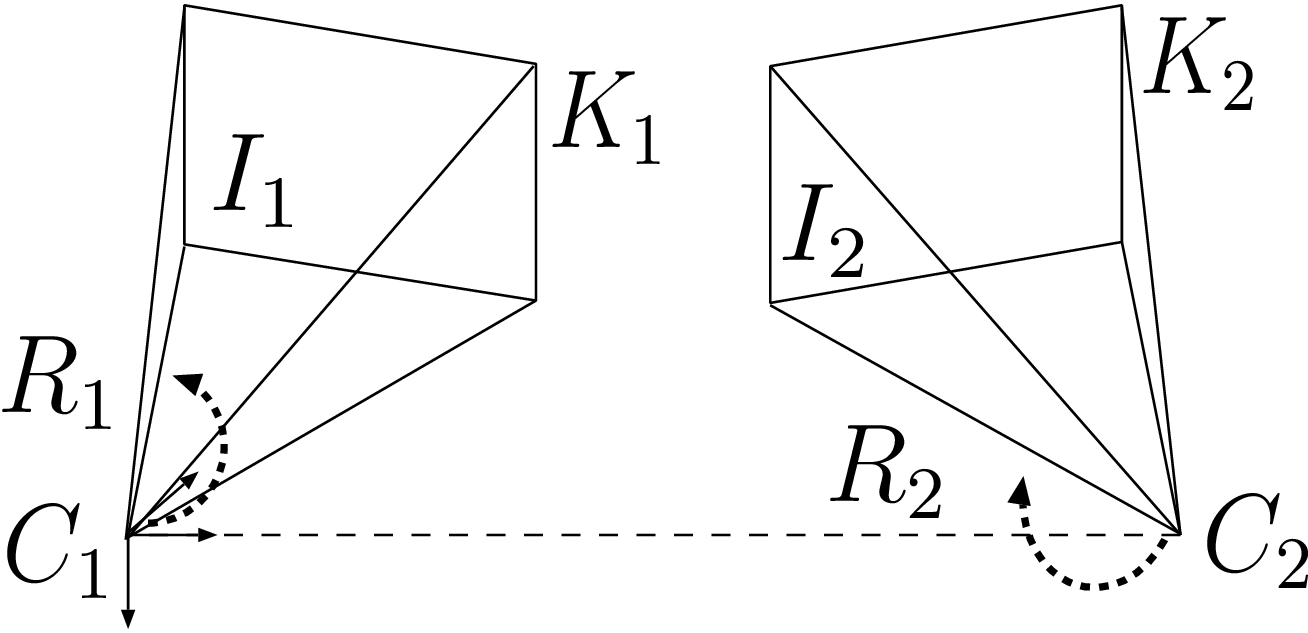
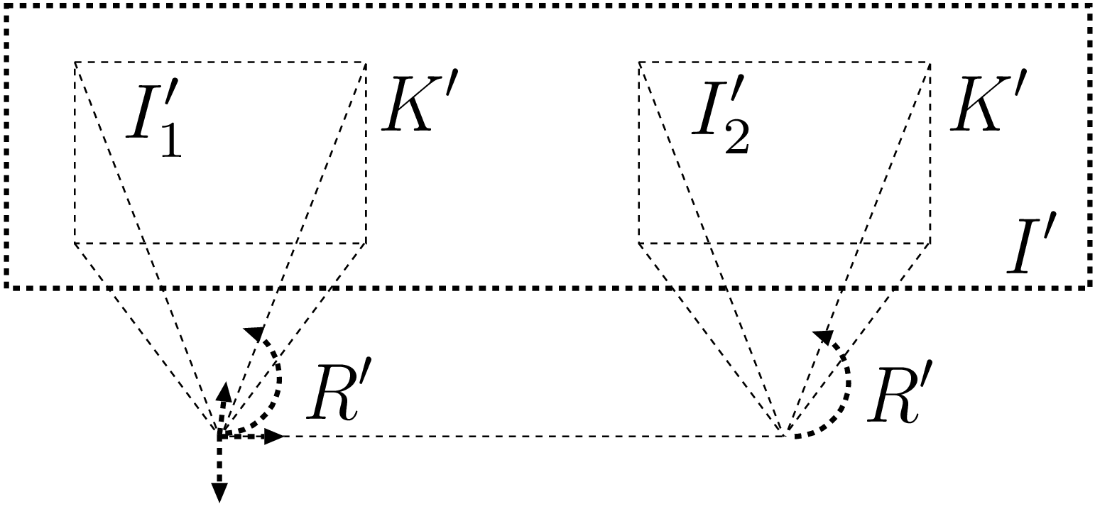
Figure 2.9 The image-rectification operation re-projects two images \(I_1\) and \(I_2\) onto a common synthetic image plane \(I'\).
We now derive the transform between the original image \(I_1\) and rectified image \(I_1'\). Let us consider a pixel \(\boldsymbol{p}_1\) and its projections on the rectified image \(\boldsymbol{p}_1'\) in \(I_1\) and \(I_1'\), respectively (illustrated by Figure 2.12). Without loss of generality, it is assumed that the camera is located at the origin of the world coordinate system.

2.12 A 3D point \((X,Y,Z)^T\) is projected onto the original and rectified image planes \(I_1\) and \(I_1'\) at pixel position \(\boldsymbol{p}_1\) and \(\boldsymbol{p}_1'\).
The projection of a 3D point \((X,Y,Z)^T\) onto the original and rectified images can be written as \[\lambda_1 \boldsymbol{p}_1 = \boldsymbol{K}_1\boldsymbol{R}_1 \left( \begin{array}{c} X\\ Y\\ Z \end{array} \right) \text{ and } \lambda_1' \boldsymbol{p}_1' = \boldsymbol{K}'\boldsymbol{R}' \left( \begin{array}{c} X\\ Y\\ Z \end{array} \right), (2.45)\] with \(\boldsymbol{R}_1,\boldsymbol{K}_1\) and \(\boldsymbol{R}',\boldsymbol{K}'\) being the original and (virtual) rectification matrices, respectively. By recombining both previous relations, we obtain the transformation between the original and rectified image planes defined as \[\frac{\lambda_1'}{\lambda_1} \boldsymbol{p}_1'=\underbrace{ \boldsymbol{K}' \boldsymbol{R}' \boldsymbol{R}_1^{-1}\boldsymbol{K}_1^{-1}}_{\boldsymbol{H}_1}\boldsymbol{p}_1. (2.44)\] Similarly, the rectification of image \(I_2\) is performed using the relation \[\frac{\lambda_2'}{\lambda_2} \boldsymbol{p}_2'=\underbrace{ \boldsymbol{K}' \boldsymbol{R}' \boldsymbol{R}_2^{-1}\boldsymbol{K}_2^{-1}}_{\boldsymbol{H}_2}\boldsymbol{p}_2. (2.45)\] When observing Equation (2.44), it can be noted that the four matrices can be combined into a \(3 \times 3\) matrix that corresponds to a homography transform. We now provide details on the computation of the rotation and projection matrix \(\boldsymbol{R}'\) and \(\boldsymbol{K}'\).
A. Calculation of matrix \(\boldsymbol{R}'\)
A single rotation matrix \(\boldsymbol{R}'\) can rotate the two cameras towards the same direction. The rotation matrix \(\boldsymbol{R}'=(\boldsymbol{r}'^x ,\boldsymbol{r}'^y ,\boldsymbol{r}'^z )^T\) can be calculated as follows.
The row \(\boldsymbol{r}'^x\) can be defined parallel to the baseline going through the two cameras centers \(\boldsymbol{C}_1\) and \(\boldsymbol{C}_2\), leading to \(\boldsymbol{r}'^x\)=\(\frac{\boldsymbol{C}_1-\boldsymbol{C}_2}{||\boldsymbol{C}_1-\boldsymbol{C}_2||}\).
The row \(\boldsymbol{r}'^y\) can be chosen as \(\boldsymbol{r}'^y=\boldsymbol{r}^{z}\times \boldsymbol{r}'^x\) where \(\boldsymbol{r}^z\) is the first row vector of the rotation matrix \(\boldsymbol{R}_1\). In this case, the new axis \(\boldsymbol{r}'^y\) is perpendicular to both the new \(\boldsymbol{r}'^x\) and the old \(\boldsymbol{r}^z\) of matrix \(\boldsymbol{R}_1\).
The row \(\boldsymbol{r}'^z\) is defined orthogonal to \(\boldsymbol{r}'^x\) and \(\boldsymbol{r}'^y\) such that \(\boldsymbol{r}'^z=\boldsymbol{r}'^x \times \boldsymbol{r}'^y\).
Note that each vector is normalized by \(\boldsymbol{r}^k:=\boldsymbol{r}^k/||\boldsymbol{r}^k||\), where \(||\boldsymbol{r}^k||\) represents the L2-Norm of the vector and \(k \in\{x,y,z\}\).
B. Calculation of matrix \(\boldsymbol{K}'\)
The intrinsic parameters of \(\boldsymbol{K}'\) must be equal for both image-rectification operations and can be defined arbitrarily, e.g., \(\boldsymbol{K}'=\frac{\boldsymbol{K}_1+\boldsymbol{K}_2}{2}\).
C. Calculation of the bounding box
Basically, Equation (2.44) means that the image rectification corresponds to a homography transform. Because a homography transforms rectangles into quadrilaterals of arbitrary size, the size of the output image needs to be calculated. The bounding box calculation needs to be carried out for both rectified images and the largest bounding box should be selected as the common bounding box. The upper-left and bottom-right corners of the two rectified images are denoted \((min_x,min_y)\) and \((max_x,max_y)\) (see Figure 2.13). Subsequently, the width and height of the output image can be written as \(w'=max_x-min_x\) and \(h'=max_y-min_y\), respectively. Additionally, as illustrated at the corner-points in Figure 2.13, some points with positive coordinates may be projected at negative pixel positions.

2.13 Bounding box calculation of the rectified images derived from a planar homography transform.
Consequently, we modify the homography transforms \(\boldsymbol{H}_1\) and \(\boldsymbol{H}_2\) to obtain new homographies \(\boldsymbol{H}_{1}'\) and \(\boldsymbol{H}_{2}'\) that map all input pixels to positive coordinates, where \(\boldsymbol{H}_{i}'\), for \(i\) is 1 or 2, can be defined by \[\begin{array}{ccc} \boldsymbol{H}'_{i}=\boldsymbol{T} \boldsymbol{H}_i & \textrm{ with }& \boldsymbol{T}= \left( \begin{array}{ccc} 1 &0 & -min_x\\ 0 & 1& -min_y\\ 0 &0 & 1\\ \end{array} \right). (2.46) \end{array}\]
The matrix \(\boldsymbol{T}\) corresponds to a translation matrix expressed in homogeneous coordinates.
D. Algorithm summary
The rectification homographies \(\boldsymbol{H}'_1\) and \(\boldsymbol{H}'_2\) can be defined as \[\begin{array}{l} \boldsymbol{H}'_1=\boldsymbol{T}\boldsymbol{K}'\boldsymbol{R}' \boldsymbol{R}_1^{-1}\boldsymbol{K}_1^{-1} \textrm{ and }\\ \boldsymbol{H}'_2=\boldsymbol{T}\boldsymbol{K}'\boldsymbol{R}' \boldsymbol{R}_2^{-1}\boldsymbol{K}_2^{-1}, (2.47)\\ \end{array}\] with \(\boldsymbol{T}\), \(\boldsymbol{R}'\), \(\boldsymbol{K}'\) defined as in the previous paragraphs. As an example, Figure 2.14 depicts two rectified images with two superimposed horizontal epipolar lines.
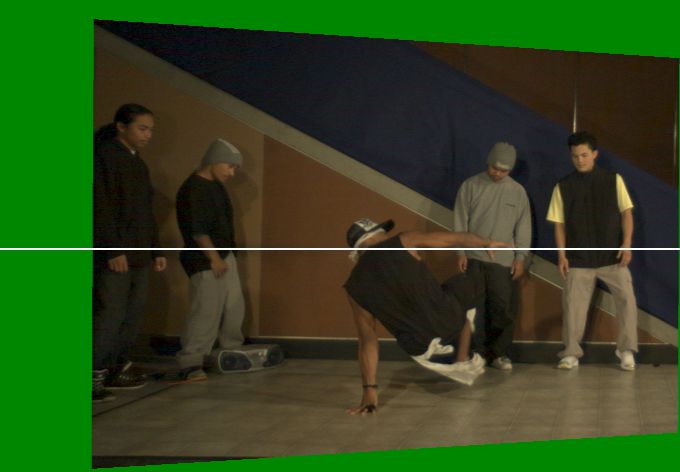

Figure 2.14 Two rectified images with two superimposed horizontal epipolar lines.
Summary and conclusions
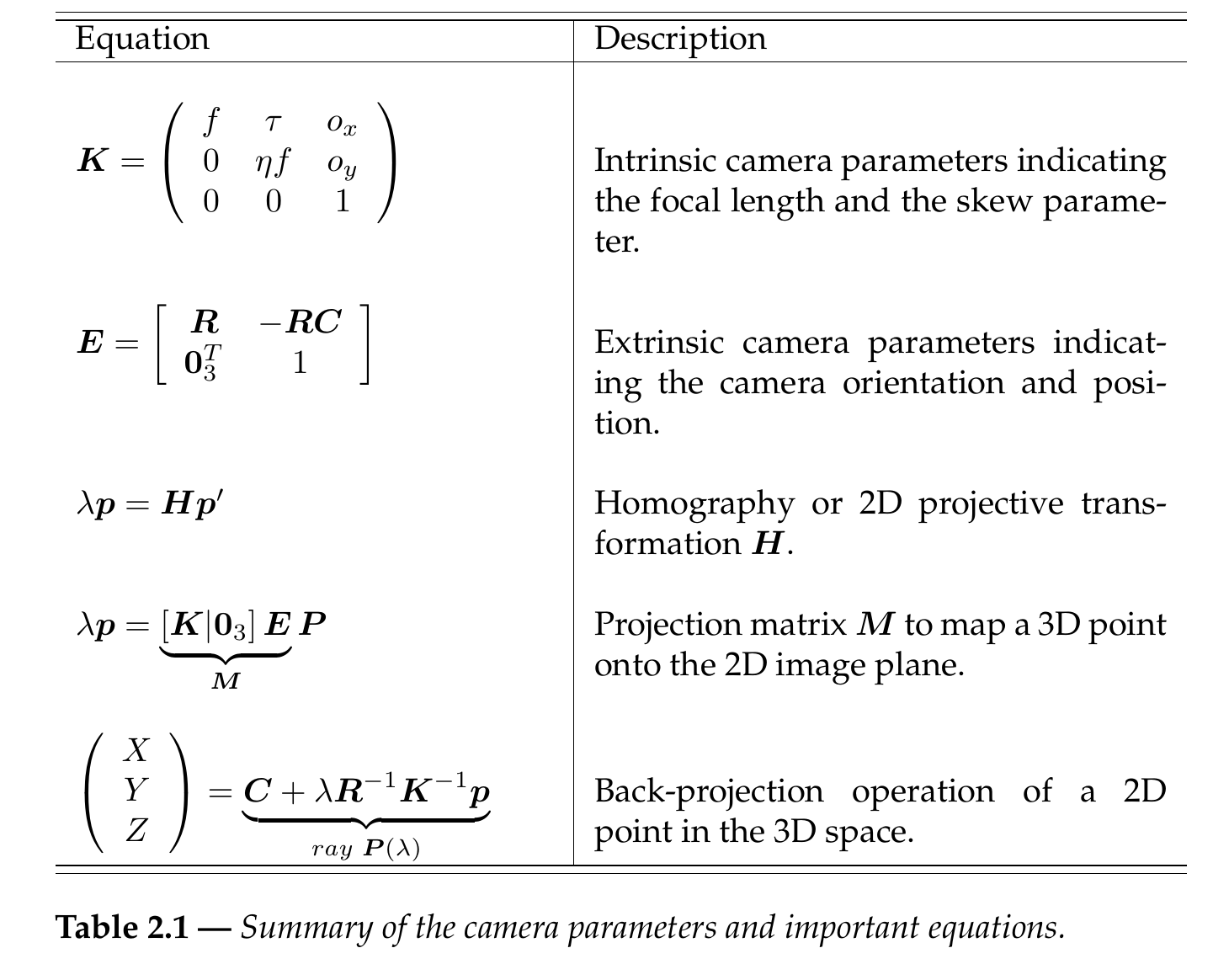
This chapter has introduced the projective geometry that uses homogeneous coordinates to represent the position of 2D and 3D points. Using homogeneous coordinates, the projection of 3D points onto the 2D image plane can be described using a linear projection matrix. We have seen that this projection matrix can be decomposed into two matrices. The first matrix \(\boldsymbol{K}\) includes the intrinsic camera parameters, comprising internal parameters such as the focal length and the principal point. The second matrix \([\boldsymbol{R}|-\boldsymbol{RC}]\) includes the extrinsic camera parameters that correspond to the position \(\boldsymbol{C}\) and orientation \(\boldsymbol{R}\) of the camera. Subsequently, the chapter has presented a flexible calibration technique that enables the estimation of the camera parameters. The camera calibration algorithm employs a planar pattern captured from, a least, three viewpoints. Finally, the two-view geometry that describes the geometric relationship between two images was introduced. For example, this two-view geometry is particularly useful to recover the 3D structure of a scene, which is a problem that is addressed in the next chapter.
A summary of camera parameters and important equations referring to epipolar geometry is presented in Table 2.1.
References
[31] T. Thormählen and H. Broszio, “Automatic line-based estimation of radial lens distortion,” Integrated Computer-Aided Engineering, vol. 12, no. 2, pp. 177–190, 2005.
[32] “Updated call for proposals on multi-view video coding.” Join Video Team ISO/IEC JTC1/SC29/WG11 MPEG2005/N7567, Nice, France, October-2005.
[33] Z. Zhang, “A flexible new technique for camera calibration,” IEEE Transactions on Pattern Analysis and Machine Intelligence, vol. 22, no. 11, pp. 1330–1334, 2000.
[34] C. Shu, A. Brunton, and M. Fiala, “Automatic grid finding in calibration patterns using delaunay triangulation,” National Research Council, Institute for Information Technology, Montreal, Canada, NRC-46497/ERB-1104, Aug. 2003.
[35] R. Hartley and A. Zisserman, Multiple view geometry in computer vision. Cambridge University Press, 2004.
[36] A. Fusiello, E. Trucco, and A. Verri, “A compact algorithm for rectification of stereo pairs,” Machine Vision and Applications, vol. 12, no. 1, pp. 16–22, 2000.